C_Meng PSNA

Never wait for the storm to pass, just dance in the rain.

0%

Chainer入门教程(下):MNIST手写体识别

III. 训练一个手写体识别器

在这一部分中,我们将使用MNIST手写数字数据集来尝试区分一个28x28像素的手写体图像。这是一个典型的有监督的深度学习。

对于这个问题,我们将会改变我们之前的线性回归器,同时引入一些隐藏的线性神经网络层,当然,也会引入一些非线性的激活函数。这种类型的架构通常被称为Multilayer Perceptron(MLP)。接下来我们就来看一下它是如何处理眼下的这个任务的。

下面的这一段代码会帮助你下载、引入并结构化MNIST数据集。然而为了完成这部分工作,你还需要下载data.py文件,并把它放在你的工作目录(你的脚本或notebook所在的目录)下以方便导入。

1
2
3
4
5
6
7
8
# functions for importing the MNIST dataset.
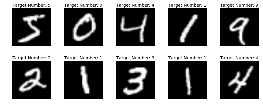
import data

# We'll first import the data as a variable mnist.
# (If this is the first time you've run this function
# it could take a minute or two)

mnist = data.load_mnist_data()

现在我们可以先看一下这些图片的样子:

1
2
3
4
5
6
7
8
9
10
plt.figure(figsize=(12,5))
for i in range(10):
example = mnist['data'][i].reshape(28, 28)
target = mnist['target'][i]
plt.subplot(2, 5, i+1)
plt.imshow(example, cmap='gray')
plt.title("Target Number: {0}".format(target))
plt.axis("off")
plt.tight_layout()
plt.show()

现在,我们要把数据集中的图像和对应的真实数字分开,并分成训练集和测试集两部分,以便我们在最后检验我们的学习成果。

1
2
3
4
5
6
7
# Separate the two parts of the MNIST dataset
features = mnist['data'].astype(np.float32) / 255
targets = mnist['target'].astype(np.int32)

# Make a train/test split.
x_train, x_test = np.split(features, [60000])
y_train, y_test = np.split(targets, [60000])

这样一来,我们就可以集中精力训练我们的MLP了。MLP包含一系列不同的layer,Chainer又有一个很不错的方法,这可以帮我们把神经网络中所有的layer都封装到一个对象中。

FunctionSet简介

这个方便的对象以命名后的layer作为关键字参数,以便我们之后可以引用它们。FunctionSet工作的方式如下:

1
model = FunctionSet(layer1=<place link here>, layer2=<place link here>, ...etc.)

然后layer就会在类的实例中作为属性存在。这些layer都可以通过把FunctionSet实例交给optimizer的setup方法同时进行优化:

1
optimizer.setup(model)

理解了这个小tip之后,我们就可以继续构建我们的分类器了。我们需要把一个28x28像素的图像降维成一个10维的单形。输出的每一个维度代表一个具体的数字。

MLP架构

为了方便教学以及理解,我们在这里建立一个只有三层的神经网络。

我们需要一个link来引入我们的28x28=784的图像,然后一步一步把它降维到10维。

另外,因为线性函数的组织是线性的,而深度学习又具有引入非线性变换的优点,所以当我们引入一些非线性函数时就会有非常好的重复线性层的堆叠。

因此,在前向传播时,我们希望线性变换层和非线性的激活函数层交替出现。通过这种方法,我们的神经网络可以学习到非线性的数据模型以得到更好的预测结果。最后我们通过一个名为softmax的交叉熵损失函数来比较输出的矢量与我们的原本提取出的答案,然后基于计算出的损失来进行反向传播。

最终我们的前向传播的架构应该是这样的形式:

1
2
3
4
5
out = linear_layer1(data)
out = relu(out)
out = linear_layer2(out)
out = relu(out)
out = linear_layer3(out)

到了训练我们的模型的时候,我们希望能够每次处理一部分的样品并在更新权重前来统计它们的损失。

Define the Model

首先,我们通过声明link的集以及在训练过程中要用到的optimizer来定义模型。

1
2
3
4
5
6
7
8
9
10
11
12
# Declare the model layers together as a FunctionSet
mnist_model = FunctionSet(
linear1=L.Linear(784, 300),
linear2=L.Linear(300, 100),
linear3=L.Linear(100, 10)
)

# Instantiate an optimizer (you should probably use an
# Adam optimizer here for best performance)
# and then setup the optimizer on the FunctionSet.
mnist_optimizer = optimizers.Adam()
mnist_optimizer.setup(mnist_model)

构造训练函数

现在我们构造一个合适的函数来进行前向传播、定义训练用的数据集以及生成训练之后对MNIST手写图像进行预测的结果。

1
2
3
4
5
6
7
8
9
10
11
12
13
14
15
16
17
18
19
20
21
22
23
24
25
26
27
28
29
30
31
32
33
34
35
36
37
38
39
40
41
42
43
# Construct a forward pass through the network,
# moving sequentially through a layer then activation function
# as stated above.
def mnist_forward(data, model):

out1 = model.linear1(data)
out2 = F.relu(out1)
out3 = model.linear2(out2)
out4 = F.relu(out3)
final = model.linear3(out4)
return final

# Make a training function which takes in training data and targets
# as an input.
def mnist_train(x, y, model, batchsize=1000, n_epochs=20):

data_size = x.shape[0]
# loop over epochs
for epoch in range(n_epochs):
print('epoch %d' % (epoch + 1))

# randomly shuffle the indices of the training data
shuffler = np.random.permutation(data_size)

# loop over batches
for i in range(0, data_size, batchsize):
x_var = Variable(x[shuffler[i : i + batchsize]])
y_var = Variable(y[shuffler[i : i + batchsize]])

output = mnist_forward(x_var, model)
model.zerograds()
loss = F.softmax_cross_entropy(output, y_var)
loss.backward()
mnist_optimizer.update()

# Make a prediction function, using a softmax and argmax in order to
# match the target space so that we can validate.
def mnist_predict(x, model):
x = Variable(x)

output = mnist_forward(x, model)

return F.softmax(output).data.argmax(1)

Train the Model

我们现在可以开始训练神经网络了(这里我们使用一个比较小的训练次数和一个比较大的批大小,这样可以帮我们节省一些训练时间。你也可以修改一些参数,说不定就会出现更好的结果呢~)

1
mnist_train(x_train, y_train, mnist_model, n_epochs=5)

进行预测

最后一件事情就是通过测试集来验证我们的模型的精确度,看看是否出现了过拟合的情况。

1
2
3
4
5
6
7
8
# Call your prediction function on the test set
pred = mnist_predict(x_test, mnist_model)

# Compare the prediction to the ground truth target values.
accuracy = (pred==y_test).mean()

# Print out test accuracy
print("Test accuracy: %f" % accuracy)

out: Test accuracy: 0.965900

可以看到,我们才训练了5次就有了一个96.59%的准确率,amazing~

模型复用

如果你觉得某一次的训练结果不错,想要保存下来以后使用,你可以通过Chainer的serializers来将其保存成hdf5格式:

1
2
serializers.save_hdf5('test.model', mnist_model)
serializers.save_hdf5('test.state', mnist_optimizer)

要调出使用的时候也很简单:

1
2
serializers.load_hdf5('my_model.model', model_name)
serializers.load_hdf5('my_optimizer.state', optimizer_name)

Conclusion

通过这篇入门教程,相信大家对于机器学习以及Chainer都有了一定的概念。可以看出,Chainer是一个非常灵活且实用的框架,机器学习也并非难以理解。如果你想进一步Chaier这个框架,个人觉得去看看Chainer的官方文档也是一个不错的选择~

Note:

本文译自:Introduction to Chainer: Neural Networks in Python

每日一句:

On n’est jamais content là où on est.(人们从来不会满意自己所在的地方。)

点击这个按钮,会有好事发生哦~(>w<)~