简介
神经网络技术在统计建模、数据的转换分类回归等各大领域都有很大的应用空间。但是由于计算本身的复杂性以及早期的计算能力不足,神经网络一直没有得到很大的发展。然而近几年,随着GPU计算的进步,涌现出一大批非常强大而实用的神经网络的训练框架如Caffe、Keras、CUDA convnet、Torch7等。在这片教程中,我们着重介绍另一款灵活又好用的框架:Chainer的基础使用方法。你可以通过Jupyter Notebook或是其他的python终端来跟进这篇教程。
在这篇教程中,我们将先通过编写一个简单的线性回归器来帮助你入门,然后我们再编写一个用于识别MNIST手写数字的标准的深度学习模型来让你熟悉编程逻辑。
首先我们需要安装几个Python包:
1 | #首先更新一下cython,旧的版本可能会导致chainer安装出错 |
I. Chainer基础
首先我们要导入这篇教程中要用到的包,关于每个包的作用,之后会有简单的介绍:
1 | #Matplotlib and Numpy |
了解Chainer中Variables和Functions的特点和作用
首先,我们通过包裹numpy数组定义两个简单的Chainer Variables变量。数组中只有一个值,这样可以方便我们后续做一些标量运算。
1 | # Create 2 chainer variables then sum their squares |
在Chainer中,Variables对象既是象征的又是数字的。它们在data属性中包含数据的值,但也包含已在它们上执行的操作链的信息。当你需要训练神经网络时,这段操作历史是非常有用的。我们通过调用backward()方法对变量进行BP或(反向模式)自动分化,这给我们提供了所选择的优化与所有更新我们的神经网络所需要的权重信息。
这个过程之所以可以发生,是因为Chainer的Variables对象把所有对其进行操作的函数都进行了存储,分析了其表达式及导数。你将会使用到的一些函数会是带参的,包含在chainer.links中(这里我们作为L导入)。这些函数的参数将在我们的网络的每个训练迭代中更新。其他包含在chainer.functions(这里我们作为F导入)中的函数将会是无参的,只是对变量执行预定义的数学操作。连加减运算都需要调用Chainer Functions,各变量的操作历史都将保存为变量本身的一部分。这使我们能够计算任何变量的相对于任何其他变量的导数。
下面我们来看一个例子,过程如下:
- 通过调用data属性检查之前定义的变量
- 使用backward()方法,对变量c进行反向传播
- 通过在变量中存储的grad属性,检查其导数
1 | #Inspect the value of your variables. |
output: a.data: [ 3.], b.data: [ 4.], c.data: [ 25.]
1 | #Now call backward() on the sum of squares. |
output: dc/da = [ 6.], dc/db = [ 8.], dc/dc = [ 1.]
II. 在Chainer中做线性回归
现在我们知道了一点关于基础的Chainer在做什么,让我们用它来训练最基本的神经网络、线性回归网络。当然,这里所涉及的最小二乘优化的解决方案,通过正常的等式计算分析可能更有效,但这个过程将展示每个网络的基本组成部分,你可以直接进行训练。
这个网络没有隐藏的节点,只涉及一个输入节点,一个输出节点,和一个连接他们两个的线性函数。
我们将要进行下列步骤:
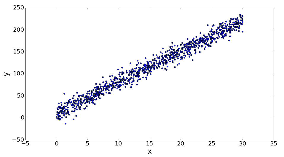
- 生成随机的线性数据集
- 通过Chainer Link构造一个前向的网络
- 构造一个函数来进行网络训练
1 | # Generate linearly related datasets x and y. |
一般来说,在Chainer中想要让你的结构保持共同的神经网络,你需要构造一个forward函数,这个函数会带入你的不同的带参的link函数并在序列中把所有数据运行一遍。
然后,我们需要写一个train函数,它将在你的所有的数据上把forward函数运行epochs次。并且在每次forward之后,都调用loss/objective函数,然后通过optimizer和通过backward方法算出的梯度来更新权重。
Chainer使用者通常会在一开始的时候就定义好Link的层(这里我们只需要一层)。然后他们会通过实例化一个optimizer类来指定要用的优化器。最后,他们会通过调用优化实例的设置方法,告诉optimizer来跟踪和更新指定的模型层的参数,该层将作为一个参数被跟踪。
1 | # Setup linear link from one variable to another. |
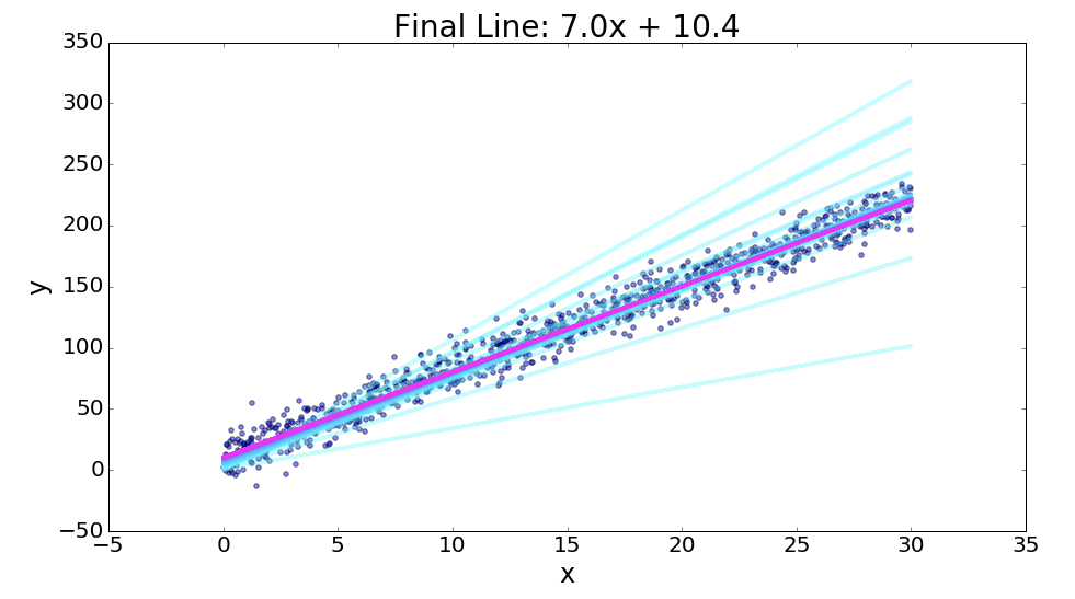
绘制训练结果
下面的代码将会把此模型每次训练5遍,并绘制线性链接中当前的参数下的线。你将会看到模型是如何从蓝色的线收敛到红色的线(最终状态)。
1 | # This code is supplied to visualize your results. |
Note:
本文译自:Introduction to Chainer: Neural Networks in Python
每日一句
Oh là là ! C’est incroyable !(艾玛,真是令人难以置信!)