reference:
https://www.researchgate.net/profile/Francisco_Ruiz14/publication/220831115_Quality_Assessment_of_Business_Process_Models_Based_on_Thresholds/links/5473100f0cf216f8cfae97f4.pdf
author:
Laura Sánchez-González, Félix García, Jan Mendling, Francisco Ruiz
Institution:
Grupo Alarcos, Universidad de Castilla La Mancha
Humboldt-Universität zu Berlin

Background and Motivation

Process improvement is recognized as the main benefit of process modelling initiatives. Quality considerations are important when conducting a process modelling project. While the early stage of business process design might not be the most expensive ones, they tend to have the highest impact on the benefits and costs of the implemented business processes. In this context, quality assurance of the models has become a significant objective.

Quality from the perspective of understandability and modifiability

The aim of our empirical research approach is to validate the connections between an extensive set of metrics (number of nodes, diameter, density, coefficient of connectivity, average gateway degree, maximum gateway degree, separability, sequentiality, depth, gateway mismatch, gateway heterogeneity, cyclicity and concurrency) and the ease with which business process models can be understood (understandability) and modified (modifiability).

null hypothesis: There is no correlation between structural metrics and understandability and modifiability

The structural metrics apparently seem to be closely connected with understandability and modifiability.

1. For understandability these include Number of Nodes, Gateway Mismatch, Depth, Coefficient of Connectivity and Sequentiality.
2. For modifiability Gateway Mismatch, Density and Sequentiality showed the best results.

Conclusion

After analyzing which measures are most useful, it is interesting to know what values of these measures indicate poor quality in models. That means, thresholds values could be used as an alarm of detecting low-quality structures in conceptual models.

The strength of the correlation of structural metrics with different quality aspects clearly shows the potential of these metrics to accurately capture aspects closely connected with actual usage.

写年度报告也好，写普通报告也好，如果能够掌握一些技巧的话，就可以给自己的报告增色不少。

绝对值，相对化

有一些数据，直接拿出来并不好看。然而如果把这些绝对值转化成相对值，比如百分比、环比、增长率等，事情就大不一样。

例子：

相对值，模糊化

有的数据已经不错了，但是老板总觉得不够好。这个时候，就需要把这些数据进行模糊化。

例子

模糊值，整合化

汇报的时候，老板通常会更在意比较“差”的部分，而这些也会直接影响你的最终评估结果。但是一年发生了这么多事情，不可能事事顺心，都表现的很好。因此需要把分散的值，整合起来。

例子：

整合值，定语化

有些时候，无论怎么整合，这些数据就是不好看。这个时候，需要在报告的数据前边加上定语，对数据进行过滤。

例子：

结语：

无论怎么套路，没做就是没做，多少就是多少，实事求是不扯谎，这是底线。

本文只是给大家提供一些年度报告的包装思路，往坏了说算是歪门邪道，充其量可以帮助大家临时抱抱佛脚。

巧妇难为无米之炊，最重要的还是平时下足功夫。把工作做好，对自己、对别人都是负责。

多一些真诚，少一些套路。

reference:
https://e-archivo.uc3m.es/bitstream/handle/10016/27943/how_MOBICOM_2018_ps.pdf?sequence=1
author:
Cristina Marquez, Marco Gramaglia, Marco Fiore, Alert Banchs, Xavier Costa-Perez
Institution:
Universidad Carlos III Madrid
CNR-IEIIT (Institute of Electronics, Computer and Telecommunication Engineering, the National Research Council of Italy)
NEC Laboratories Europe

FOR A QUICK GLANCE

What is network slicing or background

Network slicing has profound implications on resource management, as it entails an inherent trade-off between:

(i) the need for fully dedicated resources to support service customization, and

(ii) the dynamic resource sharing among services to increase resource efficiency and cost-effectiveness of the system.

Why study it or what is the problem

While the technology needed to support this paradigm is well understood from a system standpoint, its implications in terms of efficiency are still unclear.

How to do

In this paper, we fill such a gap via an empirical study of resource management efficiency in network slicing.

Building on substantial measurement data collected in an operational mobile network

(i) we quantify the efficiency gap introduced by non-reconfigurable allocation strategies of different kinds of resources, from radio access to the core of the network, and

(ii) we quantify the advantages of their dynamic orchestration at different timescales.

As a result

Our results provide insights on the achievable efficiency of network slicing architectures, their dimensioning, and their interplay with resource management algorithms.

INTRODUCTION

Background

Current trends in mobile networks point towards a strong diversification of services, which are characterized by increasingly heterogeneous Key Performance Indicator (KPI) and Quality of Service (QoS) requirements.

current mobile network architectures lack the necessary flexibility to meet the ex- treme requirements imposed by such services.

Network virtualization and slicing

The agenda for 5G networks is to achieve this mainly via network virtualization, which evolves the traditional hardbox paradigm into a cloudified architecture where the once hardware-based network functions are implemented as software Virtual Network Functions (VNFs) running on a general-purpose telco-cloud. Network virtualization enables the deployment of multiple virtual instances of the complete network, named network slices.

Network slicing strategies. Deeper slices (A to E) reserve resources to services across a wider portion of the end-to-end network architecture, but reduce the space for unconstrained resource sharing.

Network slicing and resource management

When instantiating a slice, an operator needs to allocate sufficient computational and communication resources to its VNFs. In some cases, these resources may be dedicated, be- coming inaccessible to other slices. Alternatively,

Inherent trade-off

(i) service customization, which favours the deployment of specialized slices with tailored functions for each service and, possibly, dedicated and guaranteed resources;

(ii) resource management efficiency, which increases by dynamically shar- ing the resources of the common infrastructure among the different services and slices; and,

(iii) system complexity, resulting from deploying more dynamic resource allocation mechanisms that provide higher efficiency at the cost of em- ploying elaborate operation and maintenance functions.

Contribution of this paper

From a system standpoint, the technology needed to support the different types of slices is well understood or even already available.

Our aim is to shed light on the trade-offs between customization, efficiency, and complexity in network slicing, by evaluating the impact of resource allocation dynamics at different network points. Based on our analysis, it is thus possible to determine in which cases the gains in efficiency are worth the sacrifice in customization/isolation and/or the extra complexity. Since resource management efficiency in network slicing highly depends on the traffic patterns of different services supported by the various slices, we build on substantial service-level measurement data collected by a major operator in a production mobile network, and:

(i) quantify the price paid in efficiency when suitable algorithms for dynamic resource allocation are not available, and the operator has to resort to physical network duplication;

(ii) evaluate the impact of sharing resources at different
locations of the network, including the cloudified core, the virtualized radio access, or the individual antennas;

(iii) outline the benefit of dynamic resource allocation
at different timescales, i.e., allowing to reallocate resources across slices with different reconfiguration intervals

NETWORK SCENARIO AND METRICS

Network slicing scenario

The operator owning the infrastructure implements slices $s \in S$ , each dedicated to a different subset of services. Every network level $\ell$ is composed by a set $C_{\ell}$ of network nodes.

model the mobile network architecture as a hierarchy composed by a fixed number of levels ( $\ell=1, \ldots, L$ ) ordered from the most distributed ( $\ell=1$ ) to the most centralized ( $\ell=L$ )

Slice specifications

Denote a slice specification as:

$$
\mathbb{Z}=(f, w)
$$

involves:

(i) Guaranteed time fraction $f$ : the operator engages to guarantee that the traffic demand of the slice is fully serviced during at least a fraction $f \in[0,1]$ of time.

(ii) Averaging window length w: the operator commitment on fraction f above is intended on discrete-time demands of granularity w, with traffic averaged over the disjoint time windows of duration w.

average load over window k covering a time interval of the same name with duration w:

$$
\bar{o} _ {c,s} (k)=\frac{1}{w}\int_{k}o_{c, s}(t)\mathrm{d}t
$$

the amount of resources allocated to slice s at node c during window k:

$$
r_{c, s}^{\mathbb{Z}}(k)
$$

Resource allocation to slices

Let $F _ {s, c, n} ^ {w}$ be the Cumulative Distribution Function (CDF)
of the demand for slice s at node c during reconfiguration period k, averaged over windows of length w: then, the minimum $\hat{r} _ {c, s} ^ {\mathbb{Z}} (n)$
that satisfies Equation (1) can be computed as $\hat{r} _ {c, s} ^ {\mathbb{Z}} (n)=\left(F_{s, c, n}^{w}\right)^{-1}(f)$ .

$$
\mathbb{R} _ {\ell, \tau} ^ {\mathbb{Z}} = \sum _ {s \in \mathcal{S}} \sum _ {\mathcal{C} \in C _ {\ell}} \sum_{n \in \mathcal{T}} \tau \cdot \hat{r} _ {c, s} ^ {\mathbb{Z}} (n)
$$

The above equation represents the total amount of resources needed to meet slice specifications, under the possibility of dynamically re-configuring the allocation with periodicity $\tau$ .

Multiplexing efficiency

In perfect sharing, the allocated resources correspond to those required when there is no isolation among different services, hence traffic multiplexing is maximum. Formally,

$$
\mathbb{P} _ {\ell, \tau} ^ {\mathbb{Z}} = \sum _ {c \in C_{\ell}} \sum _ {n \in \mathcal{T}} \tau \cdot \hat{r} _ {c} ^ {\mathbb{Z}} (n)
$$

Multiplexing efficiency as the ratio between the resources required with network slicing and those needed under perfect sharing:

$$
\mathbb{B} _ {\ell, \tau} ^ {\mathbb{Z}} = \mathbb{R} _ {\ell, \tau} ^ {\mathbb{Z}} / \mathbb{P} _ {\ell, \tau} ^ {\mathbb{Z}}
$$

CASE STUDIES

Our two reference urban regions are a large metropolis of
several millions of inhabitants, and a typical medium-sized city with a population of around 500,000, both situated in Europe. Service-level measurement data was collected in the target areas by a major operator with a national market share of around 30%. We leverage these real-world traffic demands to define network slices. Details are in Section 3.1.

On top of this, we model the hierarchical network infrastructures in the target regions by assuming that the operator deploys level- $\ell$ nodes so as to balance the offered load among them. This is discussed in Section 3.2.

DATA-DRIVEN EVALUATION

We organise our evaluation as follows. First, we investigate worst-case settings where very stringent slice specifications are enforced, and no dynamic reconfiguration of resources is possible (Section 4.1). We then relax these constraints, and assess efficiency as slice specifications are softened (Section 4.2), or in presence of periodic resource orchestration (Section 4.3). Finally, we evaluate the impact of varied slice configurations (Section 4.4), and of a resource assignment accounting for instantaneous traffic demands (Section 4.5).

TAKEAWAYS AND PERSPECTIVES

1. Multi-service requires more resources
2. Traffic direction is a factor
3. Loose service level agreements may not help
4. Dynamic resource assignment must also be rapid
5. Aggregating services is beneficial
6. Deployment is slightly more efficient than operation
7. Urban topography has limited impact
8. There is room for improvement

Just use:

1

pip install PyExecJS

or

1

pip3 install PyExecJS

写给自己：

1. 不管别人有没有催，不管有没有投稿日，都要给自己一个deadline
2. 想法不成熟也没关系，方法有瑕疵也没关系，总之先开始写，把想到的东西都写下来
3. 整理出第一版，就算再烂，也比没有强
4. 拿着写好内容，再去找各路大神讨论，不断优化，事半功倍

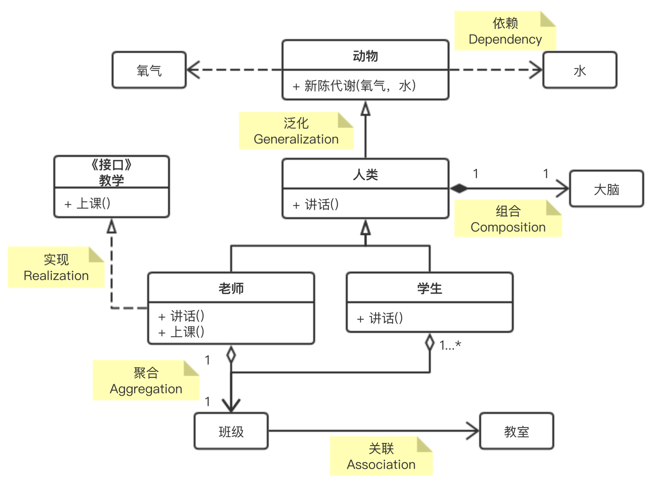
图例

说明

多目标优化是多准则决策的一个领域，它是涉及多个目标函数同时优化的数学问题。多目标优化已经应用于许多科学领域，包括工程、经济和物流，其中需要在两个或多个相互冲突的目标之间进行权衡的情况下作出最优决策。分别涉及两个和三个目标的多目标优化问题的例子有：在购买汽车时降低成本，同时使舒适性最大化；在使车辆的燃料消耗和污染物排放最小化的同时将性能最大化。在实际问题中，甚至可以有三多个目标。

对于非平凡多目标优化问题，不存在同时优化每个目标的单个解决方案。在这种情况下，目标函数被说成是冲突的，并且存在一个（可能无限）数量的帕累托最优解。如果目标函数在值上不能改进而不降低其他一些目标值，则解决方案称为非支配、Pareto最优、Pareto有效或非劣解。如果没有额外的主观偏好信息，所有Pareto最优解都被认为是同样好的（因为向量不能完全排序）。研究人员从不同的角度研究多目标优化问题，从而在设置和解决多目标优化问题时存在不同的求解哲学和目标。目标可以是找到帕累托最优解的代表性集合，and/or量化满足不同目标的折衷，and/or找到满足人类决策者decision maker(DM)的主观偏好的单一解决方案。

形式化定义

$$
\begin{array}{cl}{\min / \max } & {f_{m}(x), \quad m=1,2, \ldots, M} \\ {\text { subject to }} & {g_{j}(x) \geq 0, \quad j=1,2, \ldots, J} \\ {} & {h_{k}(x)=0, \quad k=1,2, \ldots, K} \\ {} & {x_{i}^{(Lower)} \leq x_{i} \leq x_{i}^{(Upper)}, \quad i=1,2, \ldots, n} \end{array}
$$

发展历史

多目标优化算法归结起来有传统优化算法和智能优化算法两大类。

1. 传统优化算法包括加权法、约束法和线性规划法等，实质上就是将多目标函数转化为单目标函数，通过采用单目标优化的方法达到对多目标函数的求解。
2. 智能优化算法包括进化算法（Evolutionary Algorithm, 简称EA）、粒子群算法（Particle Swarm Optimization, PSO）等。

从九十年代初开始，进化算法系列算法被统一，如遗传算法等。

多目标优化问题的解

在单目标优化问题中，通常最优解只有一个，而且能用比较简单和常用的数学方法求出其最优解。然而在多目标优化问题中，各个目标之间相互制约，可能使得一个目标性能的改善往往是以损失其它目标性能为代价，不可能存在一个使所有目标性能都达到最优的解，所以对于多目标优化问题，其解通常是一个非劣解的集合——Pareto解集。

帕累托最优（Pareto Optimal）：帕雷托最优是指资源分配的一种理想状态。给定固有的一群人和可分配的资源，如果从一种分配状态到另一种状态的变化中，在没有使任何人境况变坏的前提下，使得至少一个人变得更好，这就是帕雷托改善。帕雷托最优的状态就是不可能再有更多的帕雷托改善的状态；换句话说，不可能在不使任何其他人受损的情况下再改善某些人的境况。帕累托最优解集的边界（boundary）被称为帕累托最优前沿面（Pareto-optimal front）。

在存在多个Pareto最优解的情况下，如果没有关于问题的更多的信息，那么很难选择哪个解更可取，因此所有的Pareto最优解都可以被认为是同等重要的。由此可知，对于多目标优化问题，最重要的任务是找到尽可能多的关于该优化问题的Pareto最优解。因而，在多目标优化中主要完成以下两个任务：

1. 找到一组尽可能接近Pareto最优域的解。
2. 找到一组尽可能不同的解。

第一个任务是在任何优化工作中都必须的做到的，收敛不到接近真正Pareto最优解集的解是不可取的，只有当一组解收敛到接近真正Pareto最优解，才能确保该组解近似最优的这一特性。

几种常用的多目标优化问题解决方法

Weighted Sum Method

线性加权法，其中权重代表了每个目标函数的重要程度。

$$
\begin{array}{rl}{\min } & {F(x)=\sum_{m=1}^{M} w_{m} f_{m}(x)} \\ {\text { subject to }} & {g_{j}(x) \geq 0, \quad j=1,2, \ldots, J} \\ {} & {h_{k}(x)=0, \quad k=1,2, \ldots, K} \\ {} & {x_{i}^{(Lower)} \leq x_{i} \leq x_{i}^{(Upper)}, \quad i=1,2, \ldots, n}\end{array}
$$

优点：简单

缺点：很难设定一个权重向量能够去获得帕累托最优解；在一些非凸情况不能够保证获得帕累托最优解

$\varepsilon$ -constraint method

只保留一个目标函数，其他的目标函数被设定的值约束。

$$
\begin{array}{cl}{\min } & {f_{\mu}(x)} \\ {\text {subject to }} & {f_{m}(x) \leq \epsilon_{m}, \quad m=1,2, \ldots, M \text { and } m \neq \mu} \\ {} & {g_{j}(x) \geq 0, \quad j=1,2, \ldots, J} \\ {} & {h_{k}(x)=0,} \quad {k=1,2, \ldots, K} \\ {} & {x_{i}^{(Lower)} \leq x_{i} \leq x_{i}^{(Upper)},} \quad {i=1,2, \ldots, n}\end{array}
$$

优点：能够应用到凸函数和非凸函数场景下

缺点：函数需要精心选择；需要在独立目标函数的最小值或最大值之内

Weighted Metric Method

$$
\begin{array}{cl}{\min } & {l_{p}(x)=\left(\sum_{m=1}^{M} w_{m}\left|f_{m}(x)-z_{m}^{*}\right|\right)^{1 / p}} \\ {\text { subject to }} & {g_{j}(x) \geq 0, \quad j=1,2, \ldots, J} \\ {} & {h_{k}(x)=0, \quad k=1,2, \ldots, K} \\ {} & {x_{i}^{(Lower)} \leq x_{i} \leq x_{i}^{(Upper)}, \quad i=1,2, \ldots, n}\end{array}
$$

优点：weighted Techebycheff metirc能够保证获得所有帕累托最优解

缺点：需要有每个函数最大值和最小值的先验知识；需要每个目标函数的 $z^{*}$ 能够独立被找到；对于较小的p值，不一定保证所有能够获得所有帕累托最优解；随着p增加，问题会变得不可求导

Multi-Objective Genetic Algorithms

基于遗传算法的多目标优化就是利用遗传算法的原理来搜索帕累托最优前沿面。

遗传算法相比与传统算法的优点是能够得到一个最优解集，而不是单单一个最优解，这样给我们更多的选择。但计算复杂度可能稍高，而且里面涉及的一些函数需要精心设计。

详见：https://imonce.github.io/2019/11/07/启发式算法学习（三）：遗传算法/

发展分析

多目标优化算法相对成熟，在不同的问题使用不同的优化算法。NSGA-II, SPEA 或者 MOPSO都是可选项，而到底选择哪一个方法，还需要根据特定的情景选择。

尽管多目标优化算法应用于动态的制造系统，dynamic manufacturing systems，但是制造系统和很复杂的，并且是动态的，因此算法还是有一定的缺陷性。

未来发展方向：

1. 因为多种多目标方法已经被提出，混合方法 hybrid method可以被进一步发展。

2. 现在的动态制造系统中的多目标优化算法需要动态调度的能力

Reference:
https://www.jiqizhixin.com/graph/technologies/cf8932be-519a-4fd9-84f9-c6ffa997a554
https://blog.csdn.net/paulfeng20171114/article/details/82454310
https://hpzhao.github.io/2018/09/17/多目标优化四种方法/
https://zh.wikipedia.org/wiki/帕累托最优

算法简介

蚁群算法（Ant Colony Algorithm, AG, or Ant Colony Optimization, ACO），又称蚂蚁算法，是一种用来在图中寻找优化路径的机率型算法。它由Marco Dorigo于1992年在他的博士论文“Ant system: optimization by a colony of cooperating agents”中提出，其灵感来源于蚂蚁在寻找食物过程中发现路径的行为。蚁群算法是一种模拟进化算法，初步的研究表明该算法具有许多优良的性质。针对PID控制器参数优化设计问题，将蚁群算法设计的结果与遗传算法设计的结果进行了比较，数值仿真结果表明，蚁群算法具有一种新的模拟进化优化方法的有效性和应用价值。

基本原理

蚂蚁会在其经过的路径上释放一种可以称之为“信息素”的物质，蚁群内的蚂蚁对“信息素”具有感知能力，它们会沿着“信息素”浓度较高路径行走，而每只路过的蚂蚁都会在路上留下“信息素”，这就形成一种类似正反馈的机制，这样经过一段时间后，整个蚁群就会沿着最短路径到达食物源了。可以分解为以下几步：

1. 蚂蚁在路径上释放信息素。
2. 碰到还没走过的路口，就随机挑选一条路走。同时，释放与路径长度有关的信息素。
3. 信息素浓度与路径长度成反比。后来的蚂蚁再次碰到该路口时，就选择信息素浓度较高路径。
4. 最优路径上的信息素浓度越来越大。
5. 最终蚁群找到最优寻食路径。

算法流程

蚁群算法解决旅行商问题的流程：

数学模型

这个利用TSP问题来说明这个数学模型，对于TSP问题，设蚂蚁群体中蚂蚁的数量为m，城市的数量为n，城市i与城市j之间的距离为 $d_{ij}$ ，t时刻城市i与城市j连接路径上的信息素浓度为 $c_{ij}(t)$ 。初始时刻，蚂蚁被放置在不同的城市里，且各城市键连接路径上的信息素浓度相同。然后蚂蚁将按一定概率选择线路，不放设 $p^k_{ij}(t)$ 为t时刻蚂蚁k从城市i转移到城市j的概率。“蚂蚁TSP”策略收到两方面的左右，首先是访问某城市的期望，领完便是其他蚂蚁释放的信息素浓度。所以已定义：

$$p_{ij}^{k}(t)=\left\lbrace\begin{array}{cll}
\frac{[c_{ij}(t)]^{a} * [n_{ij}(t)]^{b}}{\sum [c_{ij}(t)]^{a} * [n_{ij}(t)]^{b}} & , & j \in allowk \\
0 & , & j \notin allowk
\end{array}\right.$$

其中：

• $n_{ij}(t)$ 为启发函数，表示蚂蚁从城市i转移到城市j的期望
• $allowk$ 为蚂蚁带访问城市集合，开始时， $allowk$ 中有 $n−1$ 个元素，即包括除了蚂蚁k出发城市的其他多个城市，随着时间的推移， $allowk$ 中的元素越来越少，直至为空
• $a$ 为信息素重要程度因子
• $b$ 为启发函数因子

在蚂蚁遍历各城市的过程中，与实际情况相似的是，在蚂蚁释放信息素的同事，各个城市之间连接路径上的信息素的强度也在通过挥发等方式逐渐消失。为了描述这个特征，设ρ表示信息素挥发程度。这样所有蚂蚁完成走完一遍所有城市之后，各个城市键连接路径上的信息素浓度为

$$c_{ij}(t+1) = (1-\rho)*c_{ij}(t) + \Delta c_{ij}$$

$$\Delta c_{ij} = \sum \Delta c^k_{ij}$$

$\Delta c^k_{ij}$ 为第k只蚂蚁在城市i与城市j连接路径上释放信息素而增加的信息素浓度。

$\Delta c_{ij}$ 为所有蚂蚁在城市i与城市j连接路径上释放信息素而增加的信息素浓度。

一般情况下 $\Delta c^k_{ij}=\frac{Q}{L_k}$ ,若蚂蚁k从城市i访问了城市j，其中 $Q$ 为信息素常数， $L_k$ 为第k只蚂蚁经过路径总长度。

python代码

代码来源：https://blog.csdn.net/fanxin_i/article/details/80380733

1
2
3
4
5
6
7
8
9
10
11
12
13
14
15
16
17
18
19
20
21
22
23
24
25
26
27
28
29
30
31
32
33
34
35
36
37
38
39
40
41
42
43
44
45
46
47
48
49
50
51
52
53
54
55
56
57
58
59
60
61
62
63
64
65
66
67
68
69
70
71
72
73
74
75
76
77
78
79
80
81
82
83
84
85
86
87
88
89
90
91
92
93
94
95
96
97
98
99
100
101
102
103
104
105
106
107
108
109
110
111
112
113
114
115
116
117
118
119
120
121
122
123
124
125
126
127
128
129
130
131
132
133
134
135
136
137
138
139
140
141
142
143
144
145
146
147
148
149
150
151
152
153
154
155
156
157
158
159
160
161
162
163
164
165
166
167
168
169
170
171
172
173
174
175
176
177
178
179
180
181
182
183
184
185
186
187
188
189
190
191
192
193
194
195
196
197
198
199
200
201
202
203
204
205
206
207
208
209
210
211
212
213
214
215
216
217
218
219
220
221
222
223
224
225
226
227
228
229
230
231
232
233
234
235
236
237
238
239
240
241
242
243
244
245
246
247
248
249
250
251
252
253
254
255
256
257
258
259
260
261
262
263
264
265
266
267
268
269
270
271
272
273
274
275
276
277
278
279
280
281
282
283
284
285
286
287
288
289
290
291
292
293
294
295
296
297
298
299
300
301
302
303
304
305
306
307
308
309
310
311
312
313
314
315
316
317
318
319
320
321
322
323
324
325

# -*- coding: utf-8 -*-
import random
import copy
import time
import sys
import math
import tkinter #//GUI模块
import threading
from functools import reduce
 
 
# 参数
'''
ALPHA:信息启发因子，值越大，则蚂蚁选择之前走过的路径可能性就越大
      ，值越小，则蚁群搜索范围就会减少，容易陷入局部最优
BETA:Beta值越大，蚁群越就容易选择局部较短路径，这时算法收敛速度会
     加快，但是随机性不高，容易得到局部的相对最优
'''
(ALPHA, BETA, RHO, Q) = (1.0,2.0,0.5,100.0)
# 城市数，蚁群
(city_num, ant_num) = (50,50)
distance_x = [
    178,272,176,171,650,499,267,703,408,437,491,74,532,
    416,626,42,271,359,163,508,229,576,147,560,35,714,
    757,517,64,314,675,690,391,628,87,240,705,699,258,
    428,614,36,360,482,666,597,209,201,492,294]
distance_y = [
    170,395,198,151,242,556,57,401,305,421,267,105,525,
    381,244,330,395,169,141,380,153,442,528,329,232,48,
    498,265,343,120,165,50,433,63,491,275,348,222,288,
    490,213,524,244,114,104,552,70,425,227,331]
#城市距离和信息素
distance_graph = [ [0.0 for col in range(city_num)] for raw in range(city_num)]
pheromone_graph = [ [1.0 for col in range(city_num)] for raw in range(city_num)]
 
 
 
#----------- 蚂蚁 -----------
class Ant(object):
 
    # 初始化
    def __init__(self,ID):
        
        self.ID = ID                 # ID
        self.__clean_data()          # 随机初始化出生点
 
    # 初始数据
    def __clean_data(self):
    
        self.path = []               # 当前蚂蚁的路径           
        self.total_distance = 0.0    # 当前路径的总距离
        self.move_count = 0          # 移动次数
        self.current_city = -1       # 当前停留的城市
        self.open_table_city = [True for i in range(city_num)] # 探索城市的状态
        
        city_index = random.randint(0,city_num-1) # 随机初始出生点
        self.current_city = city_index
        self.path.append(city_index)
        self.open_table_city[city_index] = False
        self.move_count = 1
    
    # 选择下一个城市
    def __choice_next_city(self):
        
        next_city = -1
        select_citys_prob = [0.0 for i in range(city_num)]  #存储去下个城市的概率
        total_prob = 0.0
 
        # 获取去下一个城市的概率
        for i in range(city_num):
            if self.open_table_city[i]:
                try :
                    # 计算概率：与信息素浓度成正比，与距离成反比
                    select_citys_prob[i] = pow(pheromone_graph[self.current_city][i], ALPHA) * pow((1.0/distance_graph[self.current_city][i]), BETA)
                    total_prob += select_citys_prob[i]
                except ZeroDivisionError as e:
                    print ('Ant ID: {ID}, current city: {current}, target city: {target}'.format(ID = self.ID, current = self.current_city, target = i))
                    sys.exit(1)
        
        # 轮盘选择城市
        if total_prob > 0.0:
            # 产生一个随机概率,0.0-total_prob
            temp_prob = random.uniform(0.0, total_prob)
            for i in range(city_num):
                if self.open_table_city[i]:
                    # 轮次相减
                    temp_prob -= select_citys_prob[i]
                    if temp_prob < 0.0:
                        next_city = i
                        break
 
        # 未从概率产生，顺序选择一个未访问城市
        # if next_city == -1:
        #     for i in range(city_num):
        #         if self.open_table_city[i]:
        #             next_city = i
        #             break
 
        if (next_city == -1):
            next_city = random.randint(0, city_num - 1)
            while ((self.open_table_city[next_city]) == False):  # if==False,说明已经遍历过了
                next_city = random.randint(0, city_num - 1)
 
        # 返回下一个城市序号
        return next_city
    
    # 计算路径总距离
    def __cal_total_distance(self):
        
        temp_distance = 0.0
 
        for i in range(1, city_num):
            start, end = self.path[i], self.path[i-1]
            temp_distance += distance_graph[start][end]
 
        # 回路
        end = self.path[0]
        temp_distance += distance_graph[start][end]
        self.total_distance = temp_distance
        
    
    # 移动操作
    def __move(self, next_city):
        
        self.path.append(next_city)
        self.open_table_city[next_city] = False
        self.total_distance += distance_graph[self.current_city][next_city]
        self.current_city = next_city
        self.move_count += 1
        
    # 搜索路径
    def search_path(self):
 
        # 初始化数据
        self.__clean_data()
 
        # 搜素路径，遍历完所有城市为止
        while self.move_count < city_num:
            # 移动到下一个城市
            next_city =  self.__choice_next_city()
            self.__move(next_city)
 
        # 计算路径总长度
        self.__cal_total_distance()
 
#----------- TSP问题 -----------
        
class TSP(object):
 
    def __init__(self, root, width = 800, height = 600, n = city_num):
 
        # 创建画布
        self.root = root                               
        self.width = width      
        self.height = height
        # 城市数目初始化为city_num
        self.n = n
        # tkinter.Canvas
        self.canvas = tkinter.Canvas(
                root,
                width = self.width,
                height = self.height,
                bg = "#EBEBEB",             # 背景白色 
                xscrollincrement = 1,
                yscrollincrement = 1
            )
        self.canvas.pack(expand = tkinter.YES, fill = tkinter.BOTH)
        self.title("TSP蚁群算法(n:初始化 e:开始搜索 s:停止搜索 q:退出程序)")
        self.__r = 5
        self.__lock = threading.RLock()     # 线程锁
 
        self.__bindEvents()
        self.new()
 
        # 计算城市之间的距离
        for i in range(city_num):
            for j in range(city_num):
                temp_distance = pow((distance_x[i] - distance_x[j]), 2) + pow((distance_y[i] - distance_y[j]), 2)
                temp_distance = pow(temp_distance, 0.5)
                distance_graph[i][j] =float(int(temp_distance + 0.5))
 
    # 按键响应程序
    def __bindEvents(self):
 
        self.root.bind("q", self.quite)        # 退出程序
        self.root.bind("n", self.new)          # 初始化
        self.root.bind("e", self.search_path)  # 开始搜索
        self.root.bind("s", self.stop)         # 停止搜索
 
    # 更改标题
    def title(self, s):
 
        self.root.title(s)
 
    # 初始化
    def new(self, evt = None):
 
        # 停止线程
        self.__lock.acquire()
        self.__running = False
        self.__lock.release()
 
        self.clear()     # 清除信息 
        self.nodes = []  # 节点坐标
        self.nodes2 = [] # 节点对象
 
        # 初始化城市节点
        for i in range(len(distance_x)):
            # 在画布上随机初始坐标
            x = distance_x[i]
            y = distance_y[i]
            self.nodes.append((x, y))
            # 生成节点椭圆，半径为self.__r
            node = self.canvas.create_oval(x - self.__r,
                    y - self.__r, x + self.__r, y + self.__r,
                    fill = "#ff0000",      # 填充红色
                    outline = "#000000",   # 轮廓白色
                    tags = "node",
                )
            self.nodes2.append(node)
            # 显示坐标
            self.canvas.create_text(x,y-10,              # 使用create_text方法在坐标（302，77）处绘制文字
                    text = '('+str(x)+','+str(y)+')',    # 所绘制文字的内容
                    fill = 'black'                       # 所绘制文字的颜色为灰色
                )
            
        # 顺序连接城市
        #self.line(range(city_num))
        
        # 初始城市之间的距离和信息素
        for i in range(city_num):
            for j in range(city_num):
                pheromone_graph[i][j] = 1.0
                
        self.ants = [Ant(ID) for ID in range(ant_num)]  # 初始蚁群
        self.best_ant = Ant(-1)                          # 初始最优解
        self.best_ant.total_distance = 1 << 31           # 初始最大距离
        self.iter = 1                                    # 初始化迭代次数 
            
    # 将节点按order顺序连线
    def line(self, order):
        # 删除原线
        self.canvas.delete("line")
        def line2(i1, i2):
            p1, p2 = self.nodes[i1], self.nodes[i2]
            self.canvas.create_line(p1, p2, fill = "#000000", tags = "line")
            return i2
        
        # order[-1]为初始值
        reduce(line2, order, order[-1])
 
    # 清除画布
    def clear(self):
        for item in self.canvas.find_all():
            self.canvas.delete(item)
 
    # 退出程序
    def quite(self, evt):
        self.__lock.acquire()
        self.__running = False
        self.__lock.release()
        self.root.destroy()
        print (u"\n程序已退出...")
        sys.exit()
 
    # 停止搜索
    def stop(self, evt):
        self.__lock.acquire()
        self.__running = False
        self.__lock.release()
        
    # 开始搜索
    def search_path(self, evt = None):
 
        # 开启线程
        self.__lock.acquire()
        self.__running = True
        self.__lock.release()
        
        while self.__running:
            # 遍历每一只蚂蚁
            for ant in self.ants:
                # 搜索一条路径
                ant.search_path()
                # 与当前最优蚂蚁比较
                if ant.total_distance < self.best_ant.total_distance:
                    # 更新最优解
                    self.best_ant = copy.deepcopy(ant)
            # 更新信息素
            self.__update_pheromone_gragh()
            print (u"迭代次数：",self.iter,u"最佳路径总距离：",int(self.best_ant.total_distance))
            # 连线
            self.line(self.best_ant.path)
            # 设置标题
            self.title("TSP蚁群算法(n:随机初始 e:开始搜索 s:停止搜索 q:退出程序) 迭代次数: %d" % self.iter)
            # 更新画布
            self.canvas.update()
            self.iter += 1
 
    # 更新信息素
    def __update_pheromone_gragh(self):
 
        # 获取每只蚂蚁在其路径上留下的信息素
        temp_pheromone = [[0.0 for col in range(city_num)] for raw in range(city_num)]
        for ant in self.ants:
            for i in range(1,city_num):
                start, end = ant.path[i-1], ant.path[i]
                # 在路径上的每两个相邻城市间留下信息素，与路径总距离反比
                temp_pheromone[start][end] += Q / ant.total_distance
                temp_pheromone[end][start] = temp_pheromone[start][end]
 
        # 更新所有城市之间的信息素，旧信息素衰减加上新迭代信息素
        for i in range(city_num):
            for j in range(city_num):
                pheromone_graph[i][j] = pheromone_graph[i][j] * RHO + temp_pheromone[i][j]
 
    # 主循环
    def mainloop(self):
        self.root.mainloop()
 
#----------- 程序的入口处 -----------
                
if __name__ == '__main__':
 
    TSP(tkinter.Tk()).mainloop()

Reference:
https://zh.wikipedia.org/wiki/蚁群算法
https://blog.csdn.net/fanxin_i/article/details/80380733
https://blog.csdn.net/qq_35109096/article/details/81126925st=>start: Start op1=>operation: 初始化 op15=>operation: 随机放置蚂蚁 op2=>operation: 对每只蚂蚁选择下个城市 op3=>operation: 更新信息素 op4=>operation: 输出最好路径 cond1=>condition: 还有城市可选？ cond2=>condition: 达到最大迭代次数？ ed=>end: End st->op1->op15->op2->cond1(no)->op3->cond2(yes)->ed cond1(yes)->op2 cond2(no)->op15{"scale":1,"line-width":2,"line-length":50,"text-margin":10,"font-size":12}

算法简介

遗传算法（Genetic Alogrithm，GA）是最早由美国Holland教授提出的一种基于自然界的“适者生存，优胜劣汰”基本法则的智能搜索算法。该法则很好地诠释了生物进化的自然选择过程。遗传算法也是借鉴该基本法则，通过基于种群的思想，将问题的解通过编码的方式转化为种群中的个体，并让这些个体不断地通过选择、交叉和变异算子模拟生物的进化过程，然后利用“优胜劣汰”法则选择种群中适应性较强的个体构成子种群，然后让子种群重复类似的进化过程，直到找到问题的最优解或者到达一定的进化（运算）时间。

重要概念

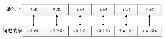
个体（染色体）：自然界中一个个体（染色体）代表一个生物，在GA算法中，个体（染色体）代表了具体问题的一个解。

基因：在GA算法中，基因代表了具体问题解的一个决策变量，问题解和染色体中基因的对应关系如下所示

种群：多个个体即组成一个种群。GA算法中，一个问题的多组解即构成了问题的解的种群。

主要步骤

主要操作介绍

种群的初始化

选择一种编码方案，然后在解空间内通过随机生成的方式初始化一定数量的个体构成GA的种群
种群的初始化和具体问题相关，一般来说可以采取某种分布（如高斯分布）在一定求解范围内随机获取

种群评价

种群的评价即计算种群中个体的适应度值。假设种群population有popsize个个体。依次计算每个个体的适应度值及评价种群。或者利用启发式算法对种群中的个体（矩形件的排入顺序）生成排样图并依此计算个体的适应函数值（利用率），然后保存当前种群中的最优个体作为搜索到的最优解。

选择操作

常见的选择操作有轮盘赌的方式：根据个体的适应度计算被选中的概率，公式如下：

$$P(x_j)=\frac{fit(x_j)}{\sum_{i=1}^n fit(x_i)}, j\in{1,2,…,n}$$

交叉操作

一般以概率阀值Pc控制是否进行单点交叉、多点交叉或者其他交叉方式生成新的交叉个体。

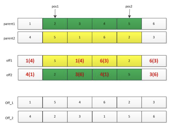
交叉操作也有许多种：单点交叉，两点交叉等。此处仅讲解一下两点交叉。首先利用选择操作从种群中选择两个父辈个体parent1和parent2,然后随机产生两个位置pos1和pos2，将这两个位置中间的基因位信息进行交换，便得到下图所示的off1和off2两个个体，但是这两个个体中一般会存在基因位信息冲突的现象（整数编码时），此时需要对off1和off2个体进行调整：off1中的冲突基因根据parent1中的基因调整为parent2中的相同位置处的基因。如off1中的“1”出现了两次，则第二处的“1”需要调整为parent1中“1”对应的parent2中的“4”，依次类推处理off1中的相冲突的基因。需要注意的是，调整off2，则需要参考parent2。

变异操作

一般以概率阀值Pm控制是否对个体的部分基因执行单点变异或多点变异。

变异操作的话，根据不同的编码方式有不同的变异操作。

如果是浮点数编码，则变异可以就染色体中间的某一个基因位的信息进行变异（重新生成或者其他调整方案）。

如果是采用整数编码方案，则一般有多种变异方法：位置变异（调换同一个体的多个基因）和符号变异（正数变负数）。

python实现

求 $f(x,y)=21.5+x\times\sin(4\times\pi\times x) + y \times\sin(20\times\pi\times y)$ 的最大值

代码来自：
https://blog.csdn.net/qq_30666517/article/details/78637255

1
2
3
4
5
6
7
8
9
10
11
12
13
14
15
16
17
18
19
20
21
22
23
24
25
26
27
28
29
30
31
32
33
34
35
36
37
38
39
40
41
42
43
44
45
46
47
48
49
50
51
52
53
54
55
56
57
58
59
60
61
62
63
64
65
66
67
68
69
70
71
72
73
74
75
76
77
78
79
80
81
82
83
84
85
86
87
88
89
90
91
92
93
94
95
96
97
98
99
100
101
102
103
104
105
106
107
108
109
110
111
112
113
114
115
116
117
118
119
120
121
122
123
124
125
126
127
128
129
130
131
132
133
134
135
136
137
138
139
140
141
142
143
144
145
146
147
148
149
150
151
152
153
154
155
156
157
158
159
160
161
162
163
164
165
166
167
168
169
170
171
172
173
174
175
176
177
178
179
180
181
182
183
184
185
186
187
188
189
190
191
192
193
194
195
196
197
198
199
200
201
202
203

# -*- coding:utf-8 -*- 
import numpy as np
from scipy.optimize import fsolve, basinhopping
import random
import timeit
 
 
# 根据解的精度确定染色体(chromosome)的长度
# 需要根据决策变量的上下边界来确定
def getEncodedLength(delta=0.0001, boundarylist=[]):
	# 每个变量的编码长度
	lengths = []
	for i in boundarylist:
		lower = i[0]
		upper = i[1]
		# lamnda 代表匿名函数f(x)=0,50代表搜索的初始解
		res = fsolve(lambda x: ((upper - lower) * 1 / delta) - 2 ** x - 1, 50)
		length = int(np.floor(res[0]))
		lengths.append(length)
	return lengths
 
 
# 随机生成初始编码种群
def getIntialPopulation(encodelength, populationSize):
	# 随机化初始种群为0
	chromosomes = np.zeros((populationSize, sum(encodelength)), dtype=np.uint8)
	for i in range(populationSize):
		chromosomes[i, :] = np.random.randint(0, 2, sum(encodelength))
	# print('chromosomes shape:', chromosomes.shape)
	return chromosomes
 
 
# 染色体解码得到表现型的解
def decodedChromosome(encodelength, chromosomes, boundarylist, delta=0.0001):
	populations = chromosomes.shape[0]
	variables = len(encodelength)
	decodedvalues = np.zeros((populations, variables))
	for k, chromosome in enumerate(chromosomes):
		chromosome = chromosome.tolist()
		start = 0
		for index, length in enumerate(encodelength):
			# 将一个染色体进行拆分，得到染色体片段
			power = length - 1
			# 解码得到的10进制数字
			demical = 0
			for i in range(start, length + start):
				demical += chromosome[i] * (2 ** power)
				power -= 1
			lower = boundarylist[index][0]
			upper = boundarylist[index][1]
			decodedvalue = lower + demical * (upper - lower) / (2 ** length - 1)
			decodedvalues[k, index] = decodedvalue
			# 开始去下一段染色体的编码
			start = length
	return decodedvalues
 
 
# 得到个体的适应度值及每个个体被选择的累积概率
def getFitnessValue(func, chromosomesdecoded):
	# 得到种群规模和决策变量的个数
	population, nums = chromosomesdecoded.shape
	# 初始化种群的适应度值为0
	fitnessvalues = np.zeros((population, 1))
	# 计算适应度值
	for i in range(population):
		fitnessvalues[i, 0] = func(chromosomesdecoded[i, :])
	# 计算每个染色体被选择的概率
	probability = fitnessvalues / np.sum(fitnessvalues)
	# 得到每个染色体被选中的累积概率
	cum_probability = np.cumsum(probability)
	return fitnessvalues, cum_probability
 
 
# 新种群选择
def selectNewPopulation(chromosomes, cum_probability):
	m, n = chromosomes.shape
	newpopulation = np.zeros((m, n), dtype=np.uint8)
	# 随机产生M个概率值
	randoms = np.random.rand(m)
	for i, randoma in enumerate(randoms):
		logical = cum_probability >= randoma
		index = np.where(logical == 1)
		# index是tuple,tuple中元素是ndarray
		newpopulation[i, :] = chromosomes[index[0][0], :]
	return newpopulation
 
 
# 新种群交叉
def crossover(population, Pc=0.8):
	"""
	:param population: 新种群
	:param Pc: 交叉概率默认是0.8
	:return: 交叉后得到的新种群
	"""
	# 根据交叉概率计算需要进行交叉的个体个数
	m, n = population.shape
	numbers = np.uint8(m * Pc)
	# 确保进行交叉的染色体个数是偶数个
	if numbers % 2 != 0:
		numbers += 1
	# 交叉后得到的新种群
	updatepopulation = np.zeros((m, n), dtype=np.uint8)
	# 产生随机索引
	index = random.sample(range(m), numbers)
	# 不进行交叉的染色体进行复制
	for i in range(m):
		if not index.__contains__(i):
			updatepopulation[i, :] = population[i, :]
	# crossover
	while len(index) > 0:
		a = index.pop()
		b = index.pop()
		# 随机产生一个交叉点
		crossoverPoint = random.sample(range(1, n), 1)
		crossoverPoint = crossoverPoint[0]
		# one-single-point crossover
		updatepopulation[a, 0:crossoverPoint] = population[a, 0:crossoverPoint]
		updatepopulation[a, crossoverPoint:] = population[b, crossoverPoint:]
		updatepopulation[b, 0:crossoverPoint] = population[b, 0:crossoverPoint]
		updatepopulation[b, crossoverPoint:] = population[a, crossoverPoint:]
	return updatepopulation
 
 
# 染色体变异
def mutation(population, Pm=0.01):
	"""
	:param population: 经交叉后得到的种群
	:param Pm: 变异概率默认是0.01
	:return: 经变异操作后的新种群
	"""
	updatepopulation = np.copy(population)
	m, n = population.shape
	# 计算需要变异的基因个数
	gene_num = np.uint8(m * n * Pm)
	# 将所有的基因按照序号进行10进制编码，则共有m*n个基因
	# 随机抽取gene_num个基因进行基本位变异
	mutationGeneIndex = random.sample(range(0, m * n), gene_num)
	# 确定每个将要变异的基因在整个染色体中的基因座(即基因的具体位置)
	for gene in mutationGeneIndex:
		# 确定变异基因位于第几个染色体
		chromosomeIndex = gene // n
		# 确定变异基因位于当前染色体的第几个基因位
		geneIndex = gene % n
		# mutation
		if updatepopulation[chromosomeIndex, geneIndex] == 0:
			updatepopulation[chromosomeIndex, geneIndex] = 1
		else:
			updatepopulation[chromosomeIndex, geneIndex] = 0
	return updatepopulation
 
 
# 定义适应度函数
def fitnessFunction():
	return lambda x: 21.5 + x[0] * np.sin(4 * np.pi * x[0]) + x[1] * np.sin(20 * np.pi * x[1])
 
 
def main(max_iter=500):
    # 每次迭代得到的最优解
    optimalSolutions = []
    optimalValues = []
    # 决策变量的取值范围
    decisionVariables = [[-3.0, 12.1], [4.1, 5.8]]
    # 得到染色体编码长度
    lengthEncode = getEncodedLength(boundarylist=decisionVariables)

    # 得到初始种群编码
    chromosomesEncoded = getIntialPopulation(lengthEncode, 10)

    for iteration in range(max_iter):
        # 种群解码
        decoded = decodedChromosome(lengthEncode, chromosomesEncoded, decisionVariables)
        # 得到个体适应度值和个体的累积概率
        evalvalues, cum_proba = getFitnessValue(fitnessFunction(), decoded)
        # 选择新的种群
        newpopulations = selectNewPopulation(chromosomesEncoded, cum_proba)
        # 进行交叉操作
        crossoverpopulation = crossover(newpopulations)
        # mutation
        mutationpopulation = mutation(crossoverpopulation)
        # 将变异后的种群解码，得到每轮迭代最终的种群
        final_decoded = decodedChromosome(lengthEncode, mutationpopulation, decisionVariables)
        # 适应度评价
        fitnessvalues, cum_individual_proba = getFitnessValue(fitnessFunction(), final_decoded)
        # 搜索每次迭代的最优解，以及最优解对应的目标函数的取值
        optimalValues.append(np.max(list(fitnessvalues)))
        index = np.where(fitnessvalues == max(list(fitnessvalues)))
        optimalSolutions.append(final_decoded[index[0][0], :])
        chromosomesEncoded = mutationpopulation

    # 搜索最优解
    optimalValue = np.max(optimalValues)
    optimalIndex = np.where(optimalValues == optimalValue)
    optimalSolution = optimalSolutions[optimalIndex[0][0]]
    return optimalSolution, optimalValue
 
 
solution, value = main()
print('最优解: x1, x2')
print(solution[0], solution[1])
print('最优目标函数值:', value)
# 测量运行时间
elapsedtime = timeit.timeit(stmt=main, number=1)
print('Searching Time Elapsed:(S)', elapsedtime)

Reference:
https://blog.csdn.net/bible_reader/article/details/72782675
https://blog.csdn.net/qq_30666517/article/details/78637255st=>start: Start op1=>operation: 种群初始化 op2=>operation: 评估种群 op3=>operation: 选择操作 op4=>operation: 直接将选中的个体作为临时个体 op5=>operation: 对选中的个体进行交叉操作，产生交叉个体 op6=>operation: 直接将所有临时个体放入下一代种群中 op7=>operation: 对临时个体进行变异操作，再投入到下一代种群中 op8=>operation: 输出最优结果 cond1=>condition: 是否进行交叉操作 cond2=>condition: 是否进行变异操作 cond3=>condition: 满足终止条件? ed=>end: End st->op1->op2->op3->cond1(no)->op4->cond2(no)->op6->cond3(yes)->op8->ed cond1(yes)->op5->cond2 cond2(yes)->op7->cond3 cond3(no)->op2{"scale":1,"line-width":2,"line-length":50,"text-margin":10,"font-size":12}