C_Meng PSNA

Never wait for the storm to pass, just dance in the rain.

0%

算法简介

模拟退火算法(Simulated annealing algorithm,SAA)的思想借鉴于固体的退火原理,当固体的温度很高的时候,内能比较大,固体的内部粒子处于快速无序运动,当温度慢慢降低的过程中,固体的内能减小,粒子的慢慢趋于有序,最终,当固体处于常温时,内能达到最小,此时,粒子最为稳定。模拟退火算法便是基于这样的原理设计而成。

模拟退火算法从某一高温出发,在高温状态下计算初始解,然后以预设的邻域函数产生一个扰动量,从而得到新的状态,即模拟粒子的无序运动,比较新旧状态下的能量,即目标函数的解。如果新状态的能量小于旧状态,则状态发生转化;如果新状态的能量大于旧状态,则以一定的概率准则发生转化。当状态稳定后,便可以看作达到了当前状态的最优解,便可以开始降温,在下一个温度继续迭代,最终达到低温的稳定状态,便得到了模拟退火算法产生的结果。

算法过程

状态空间与邻域函数

状态空间也称为搜索空间,它由经过编码的可行解的集合所组成。而邻域函数应尽可能满足产生的候选解遍布全部状态空间。其通常由产生候选解的方式和候选解产生的概率分布组成。候选解一般按照某一概率密度函数对解空间进行随机采样获得,而概率分布可以为均匀分布、正态分布、指数分布等。

状态概率分布(Metropolis准则)

状态转移概率是指从一个状态转换成另一个状态的概率,模拟退火算法中一般采用Metropolis准则,具体如下:

$$f(x)=\left\lbrace\begin{array}{cll}
1 & , & E(x_{new}) < E(x_{old}) \\
exp(-\frac{E(x_{new})-E(x_{old})}{T}) & , & E(x_{new}) \ge E(x_{old})
\end{array}\right.$$

其与当前温度参数T有关,随温度的下降而减小。

冷却进度表

冷却进度表是指从某一高温状态T向低温状态冷却时的降温函数,设时刻的温度为T(t),则经典模拟退火算法的降温方式为:

$$T(t)=\frac{T_{0}}{lg(1+t)}$$

而快速模拟退火算法的降温方式为:

$$T(t)=\frac{T_{0}}{1+t}$$

其他方法不再赘述。

初始温度

一般来说,初始温度越大,获得高质量解的几率越大,但是花费的时间也会随之增加,因此,初温的确定应该同时考虑计算效率与优化质量,常用的方法包括:

1.均匀抽样一组状态,以各状态目标值的方差为初温。

2.随机产生一组状态,确定两两状态间的最大目标值差,然后根据差值,利用一定的函数确定初温,如: $T_{0}=-\frac{\Delta_{max}}{Pr}$ ,其中Pr为初始接受概率。

3.根据经验公式给出。

循环终止准则

内循环(求解循环)终止准则:

  1. 检验目标函数的均值是否稳定
  2. 连续若干步的目标值变化较小
  3. 按一定的步数进行抽样

外循环(降温循环)终止准则:

  1. 设置终止温度
  2. 设置外循环迭代次数
  3. 算法搜索到的最优值连续若干步保持不变
  4. 检验系统熵是否稳定

Python实现

实例函数: $f(x)=(x^{2}-5x)sin(x^2)$

1
2
3
4
5
6
7
8
9
10
11
12
13
14
15
16
17
18
19
20
21
22
23
24
25
26
27
28
29
30
31
32
33
34
35
36
37
38
39
40
41
42
43
44
45
46
47
48
49
50
51
52
53
54
55
56
57
58
59
60
61
62
63
64
65
66
67
68
69
70
71
72
73
74
75
76
77
78
79
80
81
82
83
84
85
86
87
88
import numpy as np
import matplotlib.pyplot as plt
import random

class SA(object):

def __init__(self, interval, tab='min', T_max=10000, T_min=1, iterMax=1000, rate=0.95):
self.interval = interval # 给定状态空间 - 即待求解空间
self.T_max = T_max # 初始退火温度 - 温度上限
self.T_min = T_min # 截止退火温度 - 温度下限
self.iterMax = iterMax # 定温内部迭代次数
self.rate = rate # 退火降温速度

self.x_seed = random.uniform(interval[0], interval[1]) # 解空间内的种子
self.tab = tab.strip() # 求解最大值还是最小值的标签: 'min' - 最小值;'max' - 最大值

self.solve() # 完成主体的求解过程
self.display() # 数据可视化展示

def solve(self):
temp = 'deal_' + self.tab # 采用反射方法提取对应的函数
if hasattr(self, temp):
deal = getattr(self, temp)
else:
exit('>>>tab标签传参有误:"min"|"max"<<<')
x1 = self.x_seed
T = self.T_max
while T >= self.T_min:
for i in range(self.iterMax):
f1 = self.func(x1)
delta_x = random.random() * 2 - 1 # [-1,1)之间的随机值
if x1 + delta_x >= self.interval[0] and x1 + delta_x <= self.interval[1]: # 将随机解束缚在给定状态空间内
x2 = x1 + delta_x
else:
x2 = x1 - delta_x
f2 = self.func(x2)
delta_f = f2 - f1
x1 = deal(x1, x2, delta_f, T)
T *= self.rate
self.x_solu = x1 # 提取最终退火解

def func(self, x): # 状态产生函数 - 即待求解函数
value = np.sin(x**2) * (x**2 - 5*x)
return value

def p_min(self, delta, T): # 计算最小值时,容忍解的状态迁移概率
probability = np.exp(-delta/T)
return probability

def p_max(self, delta, T):
probability = np.exp(delta/T) # 计算最大值时,容忍解的状态迁移概率
return probability

def deal_min(self, x1, x2, delta, T):
if delta < 0: # 更优解
return x2
else: # 容忍解
P = self.p_min(delta, T)
if P > random.random(): return x2
else: return x1

def deal_max(self, x1, x2, delta, T):
if delta > 0: # 更优解
return x2
else: # 容忍解
P = self.p_max(delta, T)
if P > random.random(): return x2
else: return x1

def display(self):
print('seed: {}\nsolution: {}'.format(self.x_seed, self.x_solu))
plt.figure(figsize=(6, 4))
x = np.linspace(self.interval[0], self.interval[1], 300)
y = self.func(x)
plt.plot(x, y, 'g-', label='function')
plt.plot(self.x_seed, self.func(self.x_seed), 'bo', label='seed')
plt.plot(self.x_solu, self.func(self.x_solu), 'r*', label='solution')
plt.title('solution = {}'.format(self.x_solu))
plt.xlabel('x')
plt.ylabel('y')
plt.legend()
plt.savefig('SA.png', dpi=500)
plt.show()
plt.close()


if __name__ == '__main__':
SA([-5, 5], 'max')

Reference
https://www.imooc.com/article/30160
https://baike.baidu.com/item/模拟退火算法/355508?fr=aladdin
https://blog.csdn.net/google19890102/article/details/45395257
https://www.cnblogs.com/xxhbdk/p/9192750.html

算法简介

粒子群算法(Particle swarm optimization,PSO)是模拟群体智能所建立起来的一种优化算法,主要用于解决最优化问题(optimization problems)。1995年由 Eberhart和Kennedy 提出,是基于对鸟群觅食行为的研究和模拟而来的。

假设一群鸟在觅食,在觅食范围内,只在一个地方有食物,所有鸟儿都看不到食物(即不知道食物的具体位置。当然不知道了,知道了就不用觅食了),但是能闻到食物的味道(即能知道食物距离自己是远是近。鸟的嗅觉是很灵敏的)。

假设鸟与鸟之间能共享信息(即互相知道每个鸟离食物多远。这个是人工假定,实际上鸟们肯定不会也不愿意),那么最好的策略就是结合自己离食物最近的位置和鸟群中其他鸟距离食物最近的位置这2个因素综合考虑找到最好的搜索位置。

粒子群算法与《遗传算法》等进化算法有很多相似之处。也需要初始化种群,计算适应度值,通过进化进行迭代等。但是与遗传算法不同,它没有交叉,变异等进化操作。与遗传算法比较,PSO的优势在于很容易编码,需要调整的参数也很少。

核心概念

PSO有几个核心概念:

  1. 粒子(particle):一只鸟。类似于遗传算法中的个体。
  2. 种群(population):一群鸟。类似于遗传算法中的种群。
  3. 位置(position):一个粒子(鸟)当前所在的位置。
  4. 经验(best):一个粒子(鸟)自身曾经离食物最近的位置。
  5. 速度(velocity ):一个粒子(鸟)飞行的速度。
  6. 适应度(fitness):一个粒子(鸟)距离食物的远近。与遗传算法中的适应度类似。

算法过程

算法说明

两个核心公式

加速度更新公式:

$$v[i] = w * v[i] + c1 * rand() *(pbest[i] - present[i]) + c2 * rand() * (gbest - present[i])$$

其中v[i]代表第i个粒子的速度,w代表惯性权值,c1和c2表示学习参数,rand()表示在0-1之间的随机数,pbest[i]代表第i个粒子搜索到的最优值,gbest代表整个集群搜索到的最优值,present[i]代表第i个粒子的当前位置。

位置更新公式:

$$present[i]=present[i]+v[i]$$

解释说明

1.粒子数:粒子数的选取一般在20个到40个之间,但是需要具体问题具体对待,如果对于复杂问题,则需要设置更多的粒子,粒子数量越多,其搜索范围就越大。

2.惯性因子 $w$ :用来控制继承多少粒子当前的速度的,越大则对于当前速度的继承程度越小,越小则对于当前速度的继承程度越大。有些同学可能会产生疑问,是不是说反了。其实不是,从公式中可以明确看出,其值越大,则速度的改变幅度就越大,则对于粒子的当前速度继承越小;反之,速度的改变幅度越小,则对于粒子当前速度继承越大。因此如果的值越大,则解的搜索范围越大,可以提高算法的全局搜索能力,但也损失了局部搜索能力,有可能错失最优解;反之如果的值越小,则解的搜索范围也就越小,算法的全局搜索能力也就越小,容易陷入局部最优。如果是变量,则其值应该随着迭代次数的增加而减小(类似于梯度下降当中的学习率)。如果为定值,则建议在0.6到0.75之间进行选取。

3.加速常数 $c1,c2$ :通过公式一可以看出,加速常数控制着飞翔速度的计算是更加看重自身经验还是群体经验。公式一中的第二项就是自身经验的体现,加速常数可以看做是用来调整自身经验在计算粒子飞翔速度上的权重。同理是用来控制群体经验在计算粒子飞翔速度过程中的权重的。如果为0,则自身经验对于速度的计算不起作用,如果为0,则群体经验对于粒子飞翔速度的计算不起作用。的取值在学术界分歧很大主要有如下几种情况:

学者 参数取值
Clerc c1=c2=2.05
Carlisle c1=2.8, c2=1.3
Trelea w=0.6, c1=c2=1.7
Eberhart w=0.729, c1=c2=1.494

python实现

1
2
3
4
5
6
7
8
9
10
11
12
13
14
15
16
17
18
19
20
21
22
23
24
25
26
27
28
29
30
31
32
33
34
35
36
37
38
39
40
41
42
43
44
45
46
47
48
49
50
51
52
53
54
55
56
57
58
# -*- coding: utf-8 -*-
"""
f(x1,x2) = x1**2 + x2**2, x1,x2 belongs to [-10,10],求Min f
"""

import matplotlib.pyplot as plt
import numpy as np


class PSO(object):
def __init__(self, population_size, max_steps):
self.w = 0.6 # 惯性权重
self.c1 = self.c2 = 2
self.population_size = population_size # 粒子群数量
self.dim = 2 # 搜索空间的维度
self.max_steps = max_steps # 迭代次数
self.x_bound = [-10, 10] # 解空间范围
self.x = np.random.uniform(self.x_bound[0], self.x_bound[1],
(self.population_size, self.dim)) # 初始化粒子群位置
self.v = np.random.rand(self.population_size, self.dim) # 初始化粒子群速度
fitness = self.calculate_fitness(self.x)
self.p = self.x # 个体的最佳位置
self.pg = self.x[np.argmin(fitness)] # 全局最佳位置
self.individual_best_fitness = fitness # 个体的最优适应度
self.global_best_fitness = np.max(fitness) # 全局最佳适应度

def calculate_fitness(self, x):
return np.sum(np.square(x), axis=1)

def evolve(self):
fig = plt.figure()
for step in range(self.max_steps):
r1 = np.random.rand(self.population_size, self.dim)
r2 = np.random.rand(self.population_size, self.dim)
# 更新速度和权重
self.v = self.w*self.v+self.c1*r1*(self.p-self.x)+self.c2*r2*(self.pg-self.x)
self.x = self.v + self.x
plt.clf()
plt.scatter(self.x[:, 0], self.x[:, 1], s=30, color='k')
plt.xlim(self.x_bound[0], self.x_bound[1])
plt.ylim(self.x_bound[0], self.x_bound[1])
plt.pause(0.01)
# plt.ion()
# plt.show()

fitness = self.calculate_fitness(self.x)
# 需要更新的个体
update_id = np.greater(self.individual_best_fitness, fitness)
self.p[update_id] = self.x[update_id]
self.individual_best_fitness[update_id] = fitness[update_id]
# 新一代出现了更小的fitness,所以更新全局最优fitness和位置
if np.min(fitness) < self.global_best_fitness:
self.pg = self.x[np.argmin(fitness)]
self.global_best_fitness = np.min(fitness)
print('best fitness: %.5f, mean fitness: %.5f' % (self.global_best_fitness, np.mean(fitness)))

pso = PSO(10, 100)
pso.evolve()

Reference:
https://blog.csdn.net/zhaozx19950803/article/details/79854466
https://blog.csdn.net/yy2050645/article/details/80740641
https://blog.csdn.net/zj15527620802/article/details/81366105

英文: Quality of Service
中文: 服务质量
介绍: 指一个网络能够利用各种基础技术,为指定的网络通信提供更好的服务能力,是网络的一种安全机制,是用来解决网络延迟和阻塞等问题的一种技术。 通过配置QoS,对企业的网络流量进行调控,避免并管理网络拥塞,减少报文的丢失率,同时也可以为企业用户提供专用带宽或者为不同的业务(语音、视频、数据等)提供差分服务。

在正常情况下,如果网络只用于特定的无时间限制的应用系统,并不需要QoS,比如Web应用,或E-mail设置等。但是对关键应用和多媒体应用就十分必要。当网络过载或拥塞时,==QoS能确保重要业务量不受延迟或丢弃==,同时保证网络的高效运行。在RFC 3644上有对QoS的说明。

可用性(Usability)

是当用户需要时网络即能工作的时间百分比。可用性主要是设备可靠性和网络存活性相结合的结果。对它起作用的还有一些其他因素,包括软件稳定性以及网络演进或升级时不中断服务的能力。 在连续5min内,如果一个IP网络所提供的丢包率<=75%,则认为该时间段是可用的,否则是不可用的。

吞吐量(网络带宽)(Throughput)

网络带宽是指在单位时间(一般指的是1秒钟)内能传输的数据量。对IP网而言可以从帧中继网借用一些概念。根据应用和服务类型,服务水平协议(SLA)可以规定承诺信息速率(CIR)、突发信息速率(BIR)和最大突发信号长度。承诺信息速率是应该予以严格保证的,对突发信息速率可以有所限定,以在容纳预定长度突发信号的同时容纳从话音到视像以及一般数据的各种服务。一般讲,吞吐量越大越好。

时延(Latency)(Packet delay)

指一项服务从网络入口到出口的平均经过时间。许多服务,特别是话音和视像等实时服务都是高度不能容忍时延的。当时延超过200-250毫秒时,交互式会话是非常麻烦的。为了提供高质量话音和会议电视,网络设备必须能保证低的时延。
产生时延的因素很多,包括分组时延、排队时延、交换时延和传播时延。传播时延是信息通过铜线、光纤或无线链路所需的时间,它是光速的函数。在任何系统中,包括同步数字系列(SDH)、异步传输模式(ATM)和弹性分组环路(RPR),传播时延总是存在的。

时延变化(抖动)(Packet delay variation)

是指同一业务流中不同分组所呈现的时延不同。高频率的时延变化称作抖动,而低频率的时延变化称作漂移。抖动主要是由于业务流中相继分组的排队等候时间不同引起的,是对服务质量影响最大的一个问题。

​某些业务类型(特别是语音和视频等实时业务)是极其不能容忍抖动的。报文到达时间的差异将在语音或视频中造成断续;另外,抖动也会影响一些网络协议的处理,有些协议是按固定的时间间隔发送交互性报文,抖动过大就会导致协议震荡,而实际上所有传输系统都有抖动,但只要抖动在规定容差之内就不会影响服务质量,另外,可利用缓存来克服过量的抖动,但这将会增加时延。

漂移是任何同步传输系统都有的一个问题。在SDH系统中是通过严格的全网分级定时来克服漂移的。在异步系统中,漂移一般不是问题。漂移会造成基群失帧,使服务质量的要求不能满足。

丢包(Packet loss)

不管是比特丢失还是分组丢失,对分组数据业务的影响比对实时业务的影响都大。在通话期间,丢失一个比特或一个分组的信息往往用户注意不到。在视像广播期间,这在屏幕上可能造成瞬间的波形干扰,然后视像很快恢复如初。即便是用传输控制协议(TCP)传送数据也能处理丢失,因为传输控制协议允许丢失的信息重发。事实上,一种叫做随机早丢(RED)的拥塞控制机制在故意丢失分组,其目的是在流量达到设定门限时抑制TCP传输速率,减少拥塞,同时还使TCP流失去同步,以防止因速率窗口的闭合引起吞吐量摆动。但分组丢失多了,会影响传输质量。所以,要保持统计数字,当超过预定门限时就向网络管理人员告警。

丢包(packetloss)可能在所有环节中发生,例如:

  • 处理过程:路由器在收到报文的时候可能由于CPU繁忙,无法处理报文而导致丢包;
  • 排队过程:在把报文调度到队列的时候可能由于队列被装满而导致丢包;
  • 传输过程:报文在链路上传输的过程中,可能由于种种原因(如链路故障等)导致的丢包。

References:
https://blog.csdn.net/qq_25077833/article/details/53428655
https://blog.csdn.net/kakingka/article/details/45698709
https://blog.csdn.net/qq_38265137/article/details/80466737

本文主要参考官方文档https://lxml.de/tutorial.html整理,如有错误欢迎指出。

1
2
from lxml import etree
from copy import deepcopy
1
2
3
4
5
6
7
8
9
10
11
12
13
# 添加Element默认添加为根节点
root = etree.Element("root")
# 通过append添加子节点
root.append(etree.Element("child1"))
# 通过SubElement添加子节点
child2 = etree.SubElement(root, "child2")
child3 = etree.SubElement(root, "child3")
print(etree.tostring(root))
print(etree.tostring(root, pretty_print=True))
# 默认encoding是ASCII
print(etree.tostring(root, encoding='iso-8859-1'))
# 如果要把byte转成str输出的话,可以用下边的语句
print(str(etree.tostring(root, pretty_print=True),encoding='utf-8'))
b'<root><child1/><child2/><child3/></root>'
b'<root>\n  <child1/>\n  <child2/>\n  <child3/>\n</root>\n'
b"<?xml version='1.0' encoding='iso-8859-1'?>\n<root><child1/><child2/><child3/></root>"
<root>
  <child1/>
  <child2/>
  <child3/>
</root>
1
2
3
4
5
6
7
# 每个元素都是一个list
child1 = root[0]
# .tag 可以取出元素的标签
print(child1.tag, len(root))
# 大部分list方法都可以使用在element上
root.insert(0, etree.Element("child0"))
print(root[0].tag)
child1 3
child0
1
2
3
4
# 可以用list函数取出子元素的list
children = list(root)
print(root)
print(children)
<Element root at 0x107b03888>
[<Element child0 at 0x107b034c8>, <Element child1 at 0x107b03448>, <Element child2 at 0x107b038c8>, <Element child3 at 0x107b03908>]
1
2
3
4
5
6
7
# 通过长度检查element是否为叶子节点
if len(root):
print('root has children')
if len(child1):
print('child1 has children')
else:
print('child1 has no child')
root has children
child1 has no child
1
2
3
4
5
6
7
8
9
10
# 不同于普通list,赋值可能会造成元素移动
print(etree.tostring(root))
root[0] = root[-1]
print(etree.tostring(root))

# 这是普通list
l = [0,1,2,3]
print(l)
l[0] = l[-1]
print(l)
b'<root><child0/><child1/><child2/><child3/></root>'
b'<root><child3/><child1/><child2/></root>'
[0, 1, 2, 3]
[3, 1, 2, 3]
1
2
3
4
5
# 要拷贝节点,需要调用deepcopy
newroot = etree.Element('newroot')
newroot.append(deepcopy(root[1]))
print(etree.tostring(root))
print(etree.tostring(newroot))
b'<root><child3/><child1/><child2/></root>'
b'<newroot><child1/></newroot>'
1
2
3
4
# etree元素自带方法可以找到对应的父节点、前一个节点、后一个节点
print(root is child1.getparent())
print(root[0] is root[1].getprevious())
print(root[1] is root[0].getnext())
True
True
True
1
2
3
4
5
6
7
8
9
# 属性以字典方式存储
root = etree.Element("root", interesting="totally")
print(etree.tostring(root))
# 通过get方法获取属性值
print(root.get("interesting"))
print(root.get("hello"))
# 通过set方法添加属性
root.set("hello", "Huhu")
print(etree.tostring(root))
b'<root interesting="totally"/>'
totally
None
b'<root interesting="totally" hello="Huhu"/>'
1
2
3
4
5
6
7
8
9
10
11
12
13
14
15
# 字典的相关方法也可以直接使用
print(root.items(), root.keys(), root.values())

# 通过 attrib 可以直接取出属性进行操作
attributes = root.attrib
print(attributes.get("no-such-attribute"))
None
attributes["hello"] = "Guten Tag"
print(attributes["hello"])
# root中的属性一并修改
print(root.get("hello"))

# 也可以转化为纯正的dict
d = dict(root.attrib)
print(d.items())
[('interesting', 'totally'), ('hello', 'Huhu')] ['interesting', 'hello'] ['totally', 'Huhu']
None
Guten Tag
Guten Tag
dict_items([('interesting', 'totally'), ('hello', 'Guten Tag')])
1
2
3
4
5
# 元素中包含文本
root = etree.Element("root")
root.text = "Hello World"
print(root.text)
print(etree.tostring(root))
Hello World
b'<root>Hello World</root>'
1
2
3
4
5
6
7
8
9
10
11
12
13
14
# 如何添加特殊元素类似于<br/>
html = etree.Element("html")
body = etree.SubElement(html, "body")
body.text = "TEXT"

print(etree.tostring(html))

br = etree.SubElement(body, "br")
print(etree.tostring(html))

br.tail = "TAIL"
print(etree.tostring(html))
body.text = "HEAD"
print(etree.tostring(html))
b'<html><body>TEXT</body></html>'
b'<html><body>TEXT<br/></body></html>'
b'<html><body>TEXT<br/>TAIL</body></html>'
b'<html><body>HEAD<br/>TAIL</body></html>'
1
2
3
4
# tail其实属于前边元素的一部分
print(etree.tostring(br))
print(etree.tostring(br, with_tail=False))
print(etree.tostring(html, method="text"))
b'<br/>TAIL'
b'<br/>'
b'HEADTAIL'
1
2
3
# xpath方法也可以使用
print(html.xpath("string()"))
print(html.xpath("//text()"))
HEADTAIL
['HEAD', 'TAIL']
1
2
3
# 甚至可以吧xpath的方法包装成函数
build_text_list = etree.XPath("//text()") # lxml.etree only!
print(build_text_list(html))
['HEAD', 'TAIL']
1
2
3
4
5
6
7
8
9
# text也可以找爸爸
texts = build_text_list(html)
print(texts[0])

parent = texts[0].getparent()
print(parent.tag)

print(texts[1])
print(texts[1].getparent().tag)
HEAD
body
TAIL
br
1
2
3
4
# 判断一段文本是正常的文本还是tail
print(texts[0].is_text)
print(texts[1].is_text)
print(texts[1].is_tail)
True
False
True
1
2
3
4
# 但是XPath下有些方法就不行了
stringify = etree.XPath("string()")
print(stringify(html))
print(stringify(html).getparent())
HEADTAIL
None
1
2
3
4
5
6
7
8
9
# etree中的树是iterable的
root = etree.Element("root")
etree.SubElement(root, "child").text = "Child 1"
etree.SubElement(root, "child").text = "Child 2"
etree.SubElement(root, "another").text = "Child 3"

print(etree.tostring(root, pretty_print=True))
for element in root.iter():
print("%s - %s" % (element.tag, element.text))
b'<root>\n  <child>Child 1</child>\n  <child>Child 2</child>\n  <another>Child 3</another>\n</root>\n'
root - None
child - Child 1
child - Child 2
another - Child 3
1
2
3
4
5
# 可以通过在iter中添加参数,来过滤输出的tag
for element in root.iter("child"):
print("%s - %s" % (element.tag, element.text))
for element in root.iter("another", "child"):
print("%s - %s" % (element.tag, element.text))
child - Child 1
child - Child 2
child - Child 1
child - Child 2
another - Child 3
1
2
3
4
5
6
7
8
9
10
11
12
13
14
15
16
# 默认情况下,所有节点都会被遍历,如Entity、Comment等,通过添加tag参数可以避免这一点
root.append(etree.Entity("#234"))
root.append(etree.Comment("some comment"))
print(etree.tostring(root))

for element in root.iter():
if isinstance(element.tag, str):
print("%s - %s" % (element.tag, element.text))
else:
print("SPECIAL: %s - %s" % (element, element.text))

for element in root.iter(tag=etree.Element):
print("%s - %s" % (element.tag, element.text))

for element in root.iter(tag=etree.Entity):
print(element.text)
b'<root><child>Child 1</child><child>Child 2</child><another>Child 3</another>&#234;<!--some comment--></root>'
root - None
child - Child 1
child - Child 2
another - Child 3
SPECIAL: &#234; - &#234;
SPECIAL: <!--some comment--> - some comment
root - None
child - Child 1
child - Child 2
another - Child 3
&#234;
1
2
3
# 通过elementTreeName.write(filePath)可以把树写进文件或通过url传输
# 或者如果你只有elementName的话,可以这么写:
# etree.ElementTree(elementName).write(filePath)
1
2
3
4
5
6
7
# 简单粗暴的直接写xml也可以
root = etree.XML(
'<html><head/><body><p>Hello<br/>World</p></body></html>')
# 通过method参数,可以序列化为不同格式,默认method = 'xml'
print(etree.tostring(root))
print(etree.tostring(root, method='html'))
print(etree.tostring(root, method='text'))
b'<html><head/><body><p>Hello<br/>World</p></body></html>'
b'<html><head></head><body><p>Hello<br>World</p></body></html>'
b'HelloWorld'
1
2
3
4
5
6
7
8
9
10
11
12
13
14
15
16
# ElementTree class,是一个element的容器,提供了一些方法来对整个root node文档进行操作
root = etree.XML('''\
<?xml version="1.0"?>
<!DOCTYPE root SYSTEM "test" [ <!ENTITY tasty "parsnips"> ]>
<root>
<a>&tasty;</a>
</root>
''')

tree = etree.ElementTree(root)
print(tree.docinfo.xml_version)
print(tree.docinfo.doctype)

tree.docinfo.public_id = '-//W3C//DTD XHTML 1.0 Transitional//EN'
tree.docinfo.system_url = 'file://local.dtd'
print(tree.docinfo.doctype)
1.0
<!DOCTYPE root SYSTEM "test">
<!DOCTYPE root PUBLIC "-//W3C//DTD XHTML 1.0 Transitional//EN" "file://local.dtd">
1
2
print(etree.tostring(tree))
print(etree.tostring(tree.getroot()))
b'<!DOCTYPE root PUBLIC "-//W3C//DTD XHTML 1.0 Transitional//EN" "file://local.dtd" [\n<!ENTITY tasty "parsnips">\n]>\n<root>\n  <a>parsnips</a>\n</root>'
b'<root>\n  <a>parsnips</a>\n</root>'
1
2
3
4
5
6
# 解析文档中以string读入的xml
some_xml_data = "<root>data</root>"

# .fromstring函数其实和.XML差不多
root = etree.fromstring(some_xml_data)
print(etree.tostring(root))
b'<root>data</root>'
1
2
3
4
5
6
7
8
9
10
11
12
13
14
# 二进制读取解析
from io import BytesIO

some_file_or_file_like_object = BytesIO(b"<root>data</root>")
tree = etree.parse(some_file_or_file_like_object)
print(etree.tostring(tree))
# 注意:parse函数返回的是ElementTree对象,不是Element,通过getroot可以转化为Element对象
# ElementTree和Element在某些方面相似,但是方法调用上不同,比如.tag只有Element可以使用
root = tree.getroot()
print(etree.tostring(root))
try:
print("tree执行:", tree.tag)
except:
print("root执行:", root.tag)
b'<root>data</root>'
root执行: root
1
2
3
4
# parser对象
parser = etree.XMLParser(remove_blank_text=True)
root = etree.XML("<root> <a/> <b> </b> </root>", parser)
print(etree.tostring(root))
b'<root><a/><b>  </b></root>'
1
2
3
4
5
6
7
8
9
10
11
12
13
14
15
16
17
18
19
20
21
22
23
24
# Incremental parsing增量解析,比如在网络分步传输的场景下需要使用
# 方法一
class DataSource:
data = [ b"<roo", b"t><", b"a/", b"><", b"/root>" ]
def read(self, requested_size):
try:
return self.data.pop(0)
except IndexError:
return b''

tree = etree.parse(DataSource())
print(etree.tostring(tree))

# 方法二
parser = etree.XMLParser()

parser.feed("<roo")
parser.feed("t><")
parser.feed("a/")
parser.feed("><")
parser.feed("/root>")

root = parser.close()
print(etree.tostring(root))
b'<root>data</root>'
b'<root><a/></root>'
1
2
3
4
5
6
7
8
9
10
11
12
13
14
# Event-driven parsing事件驱动的解析,如只需要很大的树中的一小部分时使用
# 方法一
# iterparse默认只解析end事件
some_file_like = BytesIO(b"<root><a>data</a></root>")
for event, element in etree.iterparse(some_file_like):
print("%s, %4s, %s" % (event, element.tag, element.text))

print()

# 可以修改events参数解析所有事件
some_file_like = BytesIO(b"<root><a>data</a></root>")
for event, element in etree.iterparse(some_file_like,
events=("start", "end")):
print("%5s, %4s, %s" % (event, element.tag, element.text))
end,    a, data
end, root, None

start, root, None
start,    a, data
  end,    a, data
  end, root, None
1
2
3
4
5
6
7
8
9
10
11
12
13
14
15
16
17
18
19
20
21
22
# 方法二
class ParserTarget:
events = []
close_count = 0
def start(self, tag, attrib):
self.events.append(("start", tag, attrib))
def close(self):
events, self.events = self.events, []
self.close_count += 1
return events

parser_target = ParserTarget()

parser = etree.XMLParser(target=parser_target)
events = etree.fromstring('<root test="true"/>', parser)

print(parser_target.close_count)

for event in events:
print('event: %s - tag: %s' % (event[0], event[1]))
for attr, value in event[2].items():
print(' * %s = %s' % (attr, value))
1
event: start - tag: root
 * test = true


/Users/imonce/anaconda/lib/python3.6/site-packages/ipykernel_launcher.py:15: DeprecationWarning: inspect.getargspec() is deprecated, use inspect.signature() or inspect.getfullargspec()
  from ipykernel import kernelapp as app
1
2
3
4
events = etree.fromstring('<root test="true"/>', parser)
print(parser_target.close_count)
events = etree.fromstring('<root test="true"/>', parser)
print(parser_target.close_count)
2
3
1
2
3
4
for event in events:
print('event: %s - tag: %s' % (event[0], event[1]))
for attr, value in event[2].items():
print(' * %s = %s' % (attr, value))
event: start - tag: root
 * test = true
1
2
3
4
5
6
7
8
9
10
11
12
13
14
15
# namespace命名空间,格式为:{namespace_name}tag_name
# 一般是链接,空链接的话会 ns+编号 给一个代号
# a:b的tag名会直接报错
xhtml = etree.Element("{http://www.w3.org/1999/test}testhtml")
body = etree.SubElement(xhtml, "{http://www.w3.org/1999/test}tbody")
body.text = "Hello World"

print(etree.tostring(xhtml))

# 高贵的html
xhtml = etree.Element("{http://www.w3.org/1999/xhtml}html")
body = etree.SubElement(xhtml, "{http://www.w3.org/1999/xhtml}body")
body.text = "Hello World"

print(etree.tostring(xhtml))
b'<ns0:testhtml xmlns:ns0="http://www.w3.org/1999/test"><ns0:tbody>Hello World</ns0:tbody></ns0:testhtml>'
b'<html:html xmlns:html="http://www.w3.org/1999/xhtml"><html:body>Hello World</html:body></html:html>'
1
2
3
4
5
6
7
8
9
# 设置默认命名空间
XHTML_NAMESPACE = "http://www.w3.org/1999/xhtml"
XHTML = "{%s}" % XHTML_NAMESPACE

NSMAP = {None : XHTML_NAMESPACE} # the default namespace (no prefix)
xhtml = etree.Element(XHTML + "html", nsmap=NSMAP) # lxml only!
body = etree.SubElement(xhtml, XHTML + "body")
body.text = "Hello World"
print(etree.tostring(xhtml))
b'<html xmlns="http://www.w3.org/1999/xhtml"><body>Hello World</body></html>'
1
2
3
4
5
6
7
8
9
# QName方法,快速合成或提取namespace
tag = etree.QName('http://www.w3.org/1999/xhtml', 'html')
print(tag.localname)
print(tag.namespace)
print(tag.text)

root = etree.Element('{http://www.w3.org/1999/xhtml}html')
tag = etree.QName(root)
print(tag.localname)
html
http://www.w3.org/1999/xhtml
{http://www.w3.org/1999/xhtml}html
html
1
2
# nsmap方法,直接提取命名空间字典
print(xhtml.nsmap)
{None: 'http://www.w3.org/1999/xhtml'}
1
2
3
4
5
6
# 子元素继承父元素命名空间
root = etree.Element('root', nsmap={'a': 'http://a.b/c'})
child = etree.SubElement(root, 'child',
nsmap={'b': 'http://b.c/d'})
print(root.nsmap)
print(child.nsmap)
{'a': 'http://a.b/c'}
{'b': 'http://b.c/d', 'a': 'http://a.b/c'}
1
2
3
4
5
6
# 添加带命名空间的属性,格式为:set({namespace_name}attr_name, attr_value)
body.set(XHTML + "bgcolor", "#CCFFAA")
print(etree.tostring(xhtml))
# 注意:get的时候也要带命名空间
print(body.get("bgcolor"))
print(body.get(XHTML+"bgcolor"))
b'<html xmlns="http://www.w3.org/1999/xhtml"><body xmlns:html="http://www.w3.org/1999/xhtml" html:bgcolor="#CCFFAA">Hello World</body></html>'
None
#CCFFAA
1
2
3
4
5
6
# 也可以用XPath
find_xhtml_body = etree.ETXPath( # lxml only !
"//{%s}body" % XHTML_NAMESPACE)
results = find_xhtml_body(xhtml)

print(results[0].tag)
{http://www.w3.org/1999/xhtml}body
1
2
# iter的话也要考虑namespace
for el in xhtml.iter('{*}body'): print(el.tag)
{http://www.w3.org/1999/xhtml}body
1
2
3
4
5
6
7
8
9
10
11
12
13
14
15
16
17
18
19
20
21
22
23
# E-factory:提供一种简单紧凑的语法来生成XML和HTML
from lxml.builder import E

def CLASS(*args): # class 是python中的保留字,无法直接当做属性名
return {"class":' '.join(args)}

html = page = (
E.html( # create an Element called "html"
E.head(
E.title("This is a sample document")
),
E.body(
E.h1("Hello!", CLASS("title")),
E.p("This is a paragraph with ", E.b("bold"), " text in it!"),
E.p("This is another paragraph, with a", "\n ",
E.a("link", href="http://www.python.org"), "."),
E.p("Here are some reserved characters: <spam&egg>."),
etree.XML("<p>And finally an embedded XHTML fragment.</p>"),
)
)
)

print(str(etree.tostring(page, pretty_print=True),encoding='utf-8'))
<html>
  <head>
    <title>This is a sample document</title>
  </head>
  <body>
    <h1 class="title">Hello!</h1>
    <p>This is a paragraph with <b>bold</b> text in it!</p>
    <p>This is another paragraph, with a
      <a href="http://www.python.org">link</a>.</p>
    <p>Here are some reserved characters: &lt;spam&amp;egg&gt;.</p>
    <p>And finally an embedded XHTML fragment.</p>
  </body>
</html>
1
2
3
4
5
6
7
8
9
10
11
12
13
14
15
16
17
18
19
20
21
22
23
24
25
# 此外还有一种基于属性的方法
from lxml.builder import ElementMaker # lxml only !

E = ElementMaker(namespace="http://my.de/fault/namespace",
nsmap={'p' : "http://my.de/fault/namespace"})

DOC = E.doc
TITLE = E.title
SECTION = E.section
PAR = E.par

my_doc = DOC(
TITLE("The dog and the hog"),
SECTION(
TITLE("The dog", tType='title'),
PAR("Once upon a time, ..."),
PAR("And then ...")
),
SECTION(
TITLE("The hog"),
PAR("Sooner or later ...")
)
)

print(str(etree.tostring(my_doc, pretty_print=True),encoding='utf-8'))
<p:doc xmlns:p="http://my.de/fault/namespace">
  <p:title>The dog and the hog</p:title>
  <p:section>
    <p:title tType="title">The dog</p:title>
    <p:par>Once upon a time, ...</p:par>
    <p:par>And then ...</p:par>
  </p:section>
  <p:section>
    <p:title>The hog</p:title>
    <p:par>Sooner or later ...</p:par>
  </p:section>
</p:doc>
1
2
3
4
5
# XPath的一些例子
root = etree.XML("<root><a x='123'>aText<b/><c/><b/></a></root>")
# 找儿子(单层子节点)
print(root.find("b"))
print(root.find("a").tag)
None
a
1
2
# 找孩子(所有子节点)
print(root.find(".//b").tag)
b
1
2
# 带属性找孩子
print(root.findall(".//a[@x]")[0].tag)
a
1
2
3
4
5
6
# 通过ElementTree找路径
tree = etree.ElementTree(root)
a = root[0]
print(tree.getelementpath(a[0]))
print(tree.getelementpath(a[1]))
print(tree.getelementpath(a[2]))
a/b[1]
a/c
a/b[2]

word2vec的方法主要分为CBOW(Continuous Bag Of Words)和skip-gram(n-gram)两大类。

两种方法互为镜像。简单来说,CBOW是通过上下文预测中间值来进行训练的,skip-gram是通过中间值预测上下文来进行训练的。

这里,我们使用skip-gram的方法。

python脚本

IDE: jupyter notebook

1
2
3
4
5
6
7
8
9
10
11
12
13
14
15
16
17
18
19
20
21
22
23
24
25
26
27
28
29
30
31
32
33
34
35
36
37
38
39
40
41
42
43
44
45
46
47
48
49
50
51
52
53
54
55
56
57
58
59
60
61
62
63
64
65
66
67
68
69
70
71
72
73
74
75
76
77
78
79
80
81
82
83
84
85
86
87
88
89
90
91
92
93
94
95
96
97
98
99
100
101
102
103
104
105
106
107
108
109
110
111
112
113
114
115
116
117
118
119
120
121
122
123
124
125
126
127
128
129
130
131
132
133
134
135
136
137
138
139
140
141
142
143
144
145
146
147
148
149
150
151
152
153
154
155
156
157
158
159
160
161
162
163
164
165
166
167
168
169
170
171
172
173
174
175
176
177
178
179
180
181
182
183
184
185
186
187
188
189
190
191
192
193
194
195
196
197
198
199
200
201
202
203
204
205
206
207
208
209
210
211
212
213
214
215
216
217
218
219
220
221
from __future__ import absolute_import
from __future__ import division
from __future__ import print_function

from sklearn.manifold import TSNE
import matplotlib.pyplot as plt

import collections
import math
import os
import random
import zipfile

import numpy as np
from six.moves import urllib
from six.moves import xrange
import tensorflow as tf

class BasicPatternEmbedding:
def __init__(self):
self.url = 'http://mattmahoney.net/dc/'
self.data_index = 0

self.vocabulary_size = 5000

self.batch_size = 128
self.embedding_size = 128 # Dimension of the embedding vector.
self.skip_window = 1 # How many words to consider left and right.
self.num_skips = 2 # How many times to reuse an input to generate a label.

# We pick a random validation set to sample nearest neighbors. Here we limit the
# validation samples to the words that have a low numeric ID, which by
# construction are also the most frequent.
self.valid_size = 16 # Random set of words to evaluate similarity on.
self.valid_window = 100 # Only pick dev samples in the head of the distribution.
# choose 16 numbers from 0 to 99 randomly
self.valid_examples = np.random.choice(self.valid_window, self.valid_size, replace=False)
self.num_sampled = 64 # Number of negative examples to sample.
self.num_steps = 10001

self.final_embedding = None

self.graph = tf.Graph()

# download and verify the dataset file
def maybe_download(self, filename, expected_bytes):
# If the dataset file is not under the current path, download it directly
if not os.path.exists(filename):
filename, _ = urllib.request.urlretrieve(self.url + filename, filename)
# get dataset file infomationn
statinfo = os.stat(filename)
# verify file size
if statinfo.st_size == expected_bytes:
print('Found and verified', filename)
else:
print(statinfo.st_size)
raise Exception(
'Failed to verify ' + filename + '. Can you get to it with a browser?')
return filename

# read the data from zip into a list of strings
def read_data(self, filename):
with zipfile.ZipFile(filename) as f:
# separate by default separators, that is, all null characters, including spaces, newlines (\n), tabs (\t), etc.
data = tf.compat.as_str(f.read(f.namelist()[0])).split()
return data

# process raw inputs into a dataset
def build_dataset(self, words):
# add unknown words into count list
count = [['UNK', -1]]
# count the words list and add the pairs (word_name, number) into count list
count.extend(collections.Counter(words).most_common(self.vocabulary_size - 1))
dictionary = dict()
# create a dictionary of the words with serial number
for word, _ in count:
dictionary[word] = len(dictionary)
data = list()
unk_count = 0
# convert the word list into a number list, 0 for unknown words
for word in words:
if word in dictionary:
index = dictionary[word]
else:
index = 0
unk_count += 1
data.append(index)
# update the number of UNK
count[0][1] = unk_count
# generate a new dictionary by exchanging key and value
reversed_dictionary = dict(zip(dictionary.values(), dictionary.keys()))
return data, count, dictionary, reversed_dictionary

# function to generate a training batch for the skip-gram model
def generate_batch(self, data):
# make sure the data length is OK
assert self.batch_size % self.num_skips == 0
assert self.num_skips <= 2 * self.skip_window

batch = np.ndarray(shape=(self.batch_size), dtype=np.int32)
labels = np.ndarray(shape=(self.batch_size, 1), dtype=np.int32)
span = 2 * self.skip_window + 1 # [ skip_window target skip_window ]
# create a new double-ended queue to store the buffer
buffer = collections.deque(maxlen=span)
# data_index indicates the end point of the current window
if self.data_index + span > len(data):
data_index = 0
buffer.extend(data[self.data_index:self.data_index + span])
self.data_index += span
for i in range(self.batch_size // self.num_skips):
target = self.skip_window # target label at the center of the buffer
targets_to_avoid = [self.skip_window]
# sample num_skips batches and labels, optimizable
for j in range(self.num_skips):
while target in targets_to_avoid:
target = random.randint(0, span - 1)
# avoid sampling to the same target
targets_to_avoid.append(target)
# each batch item stands for input
batch[i * self.num_skips + j] = buffer[self.skip_window]
# each label item stands for ground truth
labels[i * self.num_skips + j, 0] = buffer[target]
if self.data_index == len(data):
buffer[:] = data[:span]
self.data_index = span
else:
buffer.append(data[self.data_index])
self.data_index += 1
# Backtrack a little bit to avoid skipping words in the end of a batch
self.data_index = self.data_index - span
return batch, labels

def train(self, data, reverse_dictionary):
with self.graph.as_default():
train_inputs = tf.placeholder(tf.int32, shape=[self.batch_size])
train_labels = tf.placeholder(tf.int32, shape=[self.batch_size, 1])
valid_dataset = tf.constant(self.valid_examples, dtype=tf.int32)

# Ops and variables pinned to the CPU
with tf.device('/cpu:0'):
# Look up embeddings for inputs.
embeddings = tf.Variable(tf.random_uniform([self.vocabulary_size, self.embedding_size], -1.0, 1.0))
# according to embeddings, the 128-dimensional vector corresponding to the input word(train inputs) was extracted
embed = tf.nn.embedding_lookup(embeddings, train_inputs)

# Construct the variables for the NCE loss
nce_weights = tf.Variable(tf.truncated_normal([self.vocabulary_size, self.embedding_size], stddev=1.0 / math.sqrt(self.embedding_size)))
nce_biases = tf.Variable(tf.zeros([self.vocabulary_size]))
# Compute the average NCE loss for the batch.
# tf.nce_loss automatically draws a new sample of the negative labels each
# time we evaluate the loss.
loss = tf.reduce_mean(
tf.nn.nce_loss(weights=nce_weights,
biases=nce_biases,
labels=train_labels,
inputs=embed,
num_sampled=self.num_sampled,
num_classes=self.vocabulary_size))

# Construct the SGD optimizer using a learning rate of 1.0.
optimizer = tf.train.GradientDescentOptimizer(1.0).minimize(loss)

# Compute the cosine similarity between minibatch examples and all embeddings.
norm = tf.sqrt(tf.reduce_sum(tf.square(embeddings), 1, keep_dims=True))
normalized_embeddings = embeddings / norm
valid_embeddings = tf.nn.embedding_lookup(normalized_embeddings, valid_dataset)
similarity = tf.matmul(valid_embeddings, normalized_embeddings, transpose_b=True)

# Add variable initializer.
init = tf.global_variables_initializer()

with tf.Session(graph = self.graph) as session:
init.run()
average_loss = 0

for step in xrange(self.num_steps):
batch_inputs, batch_labels = self.generate_batch(data)
feed_dict = {train_inputs: batch_inputs, train_labels: batch_labels}

# we perform one update step by evaluating the optimizer op (including it
# in the list of returned values for session.run()
_, loss_val = session.run([optimizer, loss], feed_dict=feed_dict)
average_loss += loss_val

if step % 2000 == 0:
if step > 0:
average_loss /= 2000
# the average loss is an estimate of the loss over the last 2000 batches.
print('Average loss at step ', step, ': ', average_loss)
average_loss = 0

# output the most similar eight words to the screen
if step % 10000 == 0:
sim = similarity.eval()
for i in xrange(self.valid_size):
valid_word = reverse_dictionary[self.valid_examples[i]]
top_k = 8 # number of nearest neighbors
nearest = (-sim[i, :]).argsort()[1:top_k + 1]
log_str = 'Nearest to %s:' % valid_word
for k in xrange(top_k):
close_word = reverse_dictionary[nearest[k]]
log_str = '%s %s,' % (log_str, close_word)
print(log_str)

self.final_embeddings = normalized_embeddings.eval()

# visualize the embeddings
def plot_with_labels(self, low_dim_embs, labels, filename='tsne.png'):
assert low_dim_embs.shape[0] >= len(labels), 'More labels than embeddings'
plt.figure(figsize=(18, 18)) # in inches
for i, label in enumerate(labels):
x, y = low_dim_embs[i, :]
plt.scatter(x, y)
plt.annotate(label,
xy=(x, y),
xytext=(5, 2),
textcoords='offset points',
ha='right',
va='bottom')
plt.show()
#plt.savefig(filename)
1
2
3
4
5
6
7
8
9
10
11
12
13
14
15
16
17
18
19
20
21
22
23
24
25
26
27
28
29
if __name__ == "__main__":
try:
bpe = BasicPatternEmbedding()
filename = bpe.maybe_download('text8.zip',31344016)
vocabulary = bpe.read_data(filename)
print('Data size', len(vocabulary))
print ('vocabulary:', vocabulary[:10])

data, count, dictionary, reverse_dictionary = bpe.build_dataset(vocabulary)
del vocabulary # Hint to reduce memory.
print('Most common words (+UNK)', count[:5])
print('Sample data', data[:10], [reverse_dictionary[i] for i in data[:10]])

batch, labels = bpe.generate_batch(data)
for i in range(8):
print(batch[i], reverse_dictionary[batch[i]], '->', labels[i, 0], reverse_dictionary[labels[i, 0]])
print (dictionary['a'], dictionary['as'], dictionary['term'])

bpe.train(data, reverse_dictionary)

tsne = TSNE(perplexity=30, n_components=2, init='pca', n_iter=5000, method='exact')
plot_only = 300
low_dim_embs = tsne.fit_transform(bpe.final_embeddings[:plot_only, :])

labels = [reverse_dictionary[i] for i in xrange(plot_only)]
bpe.plot_with_labels(low_dim_embs, labels)

except ImportError:
print('Please install sklearn, matplotlib, and scipy to show embeddings.')
Found and verified text8.zip
Data size 17005207
vocabulary: ['anarchism', 'originated', 'as', 'a', 'term', 'of', 'abuse', 'first', 'used', 'against']
Most common words (+UNK) [['UNK', 2735459], ('the', 1061396), ('of', 593677), ('and', 416629), ('one', 411764)]
Sample data [0, 3081, 12, 6, 195, 2, 3134, 46, 59, 156] ['UNK', 'originated', 'as', 'a', 'term', 'of', 'abuse', 'first', 'used', 'against']
3081 originated -> 12 as
3081 originated -> 0 UNK
12 as -> 6 a
12 as -> 3081 originated
6 a -> 195 term
6 a -> 12 as
195 term -> 2 of
195 term -> 6 a
6 12 195
Average loss at step  0 :  185.77481079101562
Nearest to it: confidence, doesn, theatre, came, gulf, cultural, sites, corps,
Nearest to use: buried, grave, observation, dust, batman, security, hungarian, opens,
Nearest to at: warrior, total, rivers, yards, reaction, extinction, exclusively, eu,
Nearest to if: emergency, present, developing, dates, life, for, pennsylvania, genesis,
Nearest to between: grant, execution, generally, power, official, interpreted, hiv, binary,
Nearest to people: unlikely, mainly, prussian, dedicated, shot, spending, dangerous, pick,
Nearest to states: forward, racing, begins, printed, follow, vacuum, study, mythology,
Nearest to by: rulers, protestant, marvel, republic, zero, letters, researchers, amiga,
Nearest to american: hit, stores, managed, practiced, intermediate, retrieved, moreover, unique,
Nearest to world: leadership, decay, culture, false, vii, et, dialogue, gave,
Nearest to but: denominations, passing, according, germans, medical, emperors, working, grant,
Nearest to an: removed, marxist, experts, ac, eugene, bones, tree, ne,
Nearest to were: coat, facing, grammar, storage, teach, covering, solomon, circuit,
Nearest to to: plant, supporting, pay, pp, shell, problem, acids, post,
Nearest to be: judah, photo, films, both, senate, woman, villages, eating,
Nearest to used: legislative, hero, private, organ, spaces, vice, top, trivia,
Average loss at step  2000 :  22.257665908694268
Average loss at step  4000 :  5.249317247629166
Average loss at step  6000 :  4.652066127896309
Average loss at step  8000 :  4.529780765414238
Average loss at step  10000 :  4.432040006399155
Nearest to it: he, came, votes, matters, doesn, whole, confidence, continues,
Nearest to use: alien, buried, security, hungarian, grave, dust, batman, amount,
Nearest to at: in, killed, appearance, extinction, mathbf, rivers, eu, pronunciation,
Nearest to if: life, molecules, emergency, dates, present, pennsylvania, for, rates,
Nearest to between: eight, execution, vs, of, hiv, grant, official, documentary,
Nearest to people: UNK, mainly, dedicated, selection, unlikely, shot, fact, dangerous,
Nearest to states: forward, racing, cover, arithmetic, study, vacuum, vs, begins,
Nearest to by: and, as, in, infant, co, manufacturer, with, campaign,
Nearest to american: hit, importance, austin, entry, depending, retrieved, vs, intermediate,
Nearest to world: culture, leadership, UNK, false, mathbf, skills, et, titled,
Nearest to but: and, medical, working, was, connecticut, vs, europeans, denominations,
Nearest to an: the, ac, plant, challenge, experts, necessary, lake, marxist,
Nearest to were: jpg, are, facing, covering, manual, circuit, opposite, test,
Nearest to to: ends, and, plant, in, office, into, supporting, agave,
Nearest to be: iso, shorter, judah, self, painter, also, dependent, assistance,
Nearest to used: opposition, hero, private, illinois, legislative, regime, breaking, repeated,

相关函数说明

Tensor.eval()

.eval() 其实就是tf.Tensor的Session.run() 的另外一种写法,但两者有差别

  1. eval(): 将字符串string对象转化为有效的表达式参与求值运算返回计算结果
  2. eval()也是启动计算的一种方式。基于Tensorflow的基本原理,首先需要定义图,然后计算图,其中计算图的函数常见的有run()函数,如sess.run()。同样eval()也是此类函数,
  3. 要注意的是,eval()只能用于tf.Tensor类对象,也就是有输出的Operation,写作Tensor.eval()。对于没有输出的Operation, 可以用.run()或者Session.run();Session.run()没有这个限制。

np.argsort()

argsort函数返回的是数组值从小到大的索引值

1
2
3
>>> x = np.array([3, 1, 2])
>>> np.argsort(x)
array([1, 2, 0])

tf.reduce_sum()

reduce_sum( ) 是求和函数,在 tensorflow 里面,计算的都是 tensor,可以通过调整 axis =0,1 的维度来控制求和维度。

1
2
3
4
5
6
7
8
9
10
11
>>> x = tf.constant([[1,1,1],[1,1,1]])
>>> tf.reduce_sum(x)
6
>>> tf.reduce_sum(x, 0)
[2,2,2]
>>> tf.reduce_sum(x, 1)
[3,3]
>>> tf.reduce_sum(x, 1, keepdims=True)
[[3],[3]]
>>> tf.reduce_sum(x, [0,1])
6

tf.nn.nce_loss()

假设nce_loss之前的输入数据是K维的,一共有N个类,那么

weight.shape = (N, K)

bias.shape = (N)

inputs.shape = (batch_size, K)

labels.shape = (batch_size, num_true)

num_true : 实际的正样本个数

num_sampled: 采样出多少个负样本

num_classes = N

sampled_values: 采样出的负样本,如果是None,就会用不同的sampler去采样。待会儿说sampler是什么。

remove_accidental_hits: 如果采样时不小心采样到的负样本刚好是正样本,要不要干掉

partition_strategy:对weights进行embedding_lookup时并行查表时的策略。TF的embeding_lookup是在CPU里实现的,这里需要考虑多线程查表时的锁的问题

nce_loss的实现逻辑如下:

_compute_sampled_logits: 通过这个函数计算出正样本和采样出的负样本对应的output和label

sigmoid_cross_entropy_with_logits: 通过 sigmoid cross entropy来计算output和label的loss,从而进行反向传播。这个函数把最后的问题转化为了num_sampled+num_real个两类分类问题,然后每个分类问题用了交叉熵的损伤函数,也就是logistic regression常用的损失函数。TF里还提供了一个softmax_cross_entropy_with_logits的函数,和这个有所区别。

在训练过程中,作为input的embed也会被自动更新

tf.nn.embedding_lookup()

1
2
3
4
# Signature:
tf.nn.embedding_lookup(params, ids, partition_strategy='mod', name=None, validate_indices=True, max_norm=None)
# Docstring:
# Looks up `ids` in a list of embedding tensors.

是根据 ids 中的id,寻找 params 中的第id行。比如 ids=[1,3,5],则找出params中第1,3,5行,组成一个tensor返回。

embedding_lookup不是简单的查表,params 对应的向量是可以训练的,训练参数个数应该是 feature_num * embedding_size,即前文表述的embedding层权重矩阵,就是说 lookup 的是一种全连接层。

partition_strategy 为张量编号方式,在张量存在多维时起作用,编号的方式有两种,”mod”(默认) 和 “div”。

假设:一共有三个tensor [a,b,c] 作为params 参数,所有tensor的第 0 维上一共有 10 个项目(id 0 ~ 9)。

“mod” : (id) mod len(params) 得到 多少就把 id 分到第几个tensor里面

  • a 依次分到id: 0 3 6 9
  • b 依次分到id: 1 4 7
  • c 依次分到id: 2 5 8

“div” : (id) div len(params) 可以理解为依次排序,但是这两种切分方式在无法均匀切分的情况下都是将前(max_id+1)%len(params)个 partition 多分配一个元素.

  • a 依次分到id: 0 1 2 3
  • b 依次分到id: 4 5 6
  • c 依次分到id: 7 8 9

tf.SparseTensor()

构造稀疏向量矩阵,每一行为一个样本

SparseTensor(indices, values, dense_shape)

1
2
3
4
5
6
7
SparseTensor(indices=[[0, 0], [1, 2]], values=[1, 2], dense_shape=[3, 4])

# represents the dense tensor

[[1, 0, 0, 0]
[0, 0, 2, 0]
[0, 0, 0, 0]]

reference:
https://blog.csdn.net/qoopqpqp/article/details/76037334
https://segmentfault.com/a/1190000015287066?utm_source=tag-newest
https://blog.csdn.net/u012193416/article/details/83349138
https://blog.csdn.net/qq_36092251/article/details/79684721
https://gshtime.github.io/2018/06/01/tensorflow-embedding-lookup-sparse/

背景

柯里-霍华德同构,Curry-Howard Isomorphism,又称柯里-霍华德对应(Curry-Howard correspondence)是在计算机程序和数学证明之间的紧密联系;这种对应也叫做公式为类型对应或命题为类型对应。这是对形式逻辑系统和公式计算(computational calculus)之间符号的相似性的推广。命名来自它的两位发现者:美国数学家哈斯凯尔·柯里和逻辑学家威廉·阿尔文·霍瓦德

同构对应

Curry-Howard 同构显示了推理系统和程序语言之间的相似性,在此框架下:

  • 程序语言的语言构造同构为推理系统的推理规则
  • 程序的类型同构为逻辑命题
  • 闭合程序(不依赖环境的程序)可以同构为一条定理的证明过程,其类型就是一条定理
  • 逻辑上下文同构为自由变量类型指派
  • Lambda 演算同构为 Gentzen 的自然演绎
    • 函数调用就是蕴含消除
    • 函数抽象就是蕴含介入
    • 参数多态就是全称量化
    • 模板类型就是谓词
    • 结构类型就是合取
    • 联合类型就是析取
    • 收参数但不返回就是否定
    • call/cc 就是双重否定消除
  • SK 组合子演算同构为直觉 Hilbert 推理系统
    • S 和 K 就是演算系统的两条公理

Curry-Howard 同构与 Martin-Löf 类型论系统

这个框架里灵活性最高的是 Martin-Löf 的系统,两个高度抽象的算子—— $\prod$ 和 $\sum$ 进一步泛化了函数调用与合取,这使得它有极其恐怖的抽象能力。这个系统的推理规则是一下几条:

Introduction rule for $\prod$

$$\frac{\Gamma,x:A\vdash b:B}{\Gamma\vdash\lambda x.b:(\prod x:A)B}(\prod I)$$

Elimination rule for $\prod$

$$\frac{\Gamma\vdash f:(\prod x:A)B\quad\Gamma\vdash a:A}{\Gamma\vdash apply(f,a):B[a/x]}(\prod E)$$

Suppose $f = \lambda x.x$, then $apply(f,a)=(\lambda x.x)a$

Introduction rule for $\sum$

$$\frac{\Gamma\vdash a:A\quad\Gamma\vdash b:B[a/x]}{\Gamma\vdash\lt a,b\gt:(\sum x:A)B}(\sum I)$$

Elimination rule for $\sum$

$$\frac{\Gamma\vdash c:(\sum x:A)B\quad\Gamma,x:A,y:B\vdash d:C[\lt x,y\gt/z]}{\Gamma\vdash split(c,\lambda x.\lambda y.d):C[c/z]}(\sum E)$$

where: $split(\lt a,b\gt,\lambda x.\lambda y.d)=(\lambda x.\lambda y.d)(a)(b)$

reference
https://www.zhihu.com/question/22959608/answer/24770830
https://zh.wikipedia.org/zh-hans/柯里-霍华德同构
http://www2.math.uu.se/~palmgren/tillog/klogik04-01eng.pdf

overall

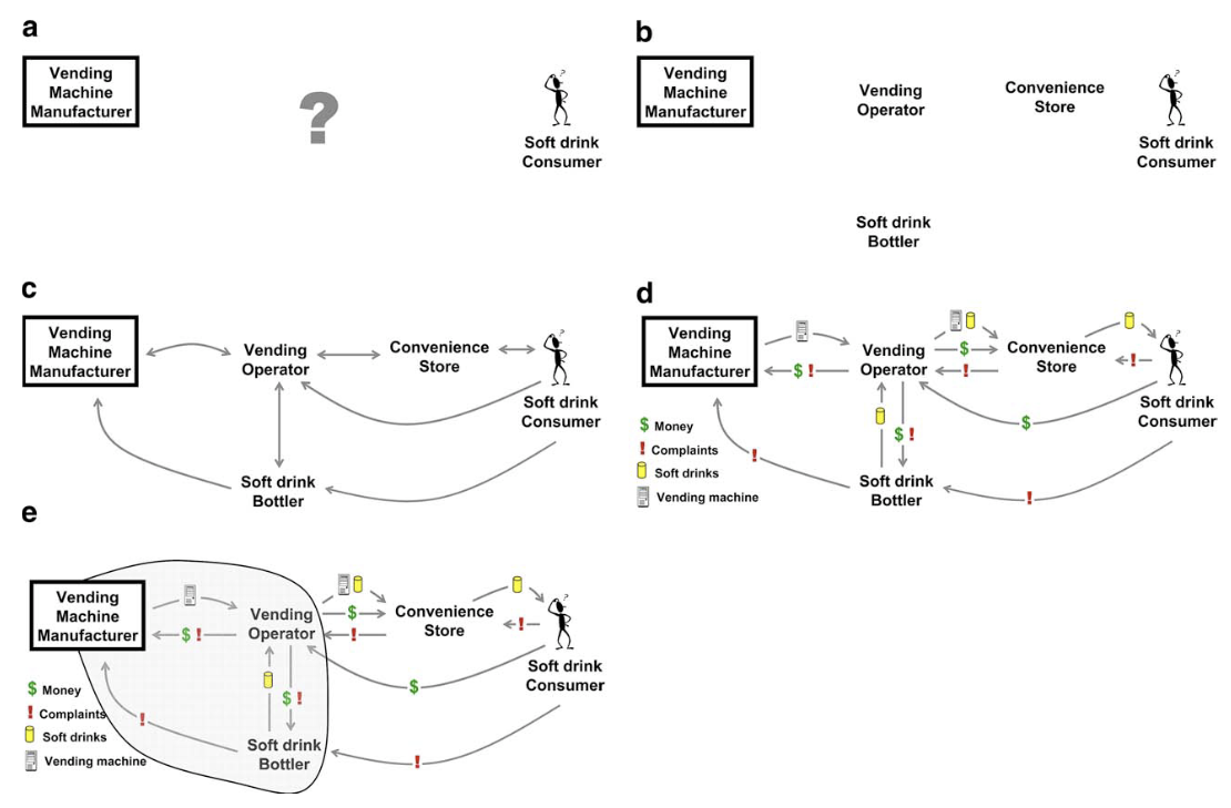
Customer Value Chain Analysis (CVCA) is an original methodological tool that enables design teams in the product definition phase to comprehensively identify pertinent stakeholders, their relationships with each other, and their role in the product’s life cycle.

method

  1. CVCA Step 1: Determine the business model for the vending machine.
  2. CVCA Step 2: Delineate pertinent parties involved with the vending machine’s life cycle.
  3. CVCA Step 3: Determine how the vending machine’s customers are related to each other.
  4. CVCA Step 4: Identify the value propositions of the vending machine’s customers and define the flows between them.
  5. CVCA Step 5: Analyze the Customer Chain to determine the vending machine’s critical customers and their value propositions. The vending operator and the soft drink bottler (circled) were determined to be the critical customers to the vending machine manufacturer.

case study

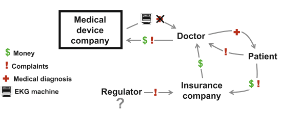
Case study 1: electrocardiogram (EKG) machine

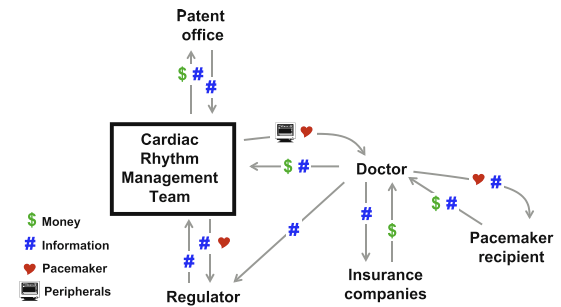
Case study 2: pacemaker alert system

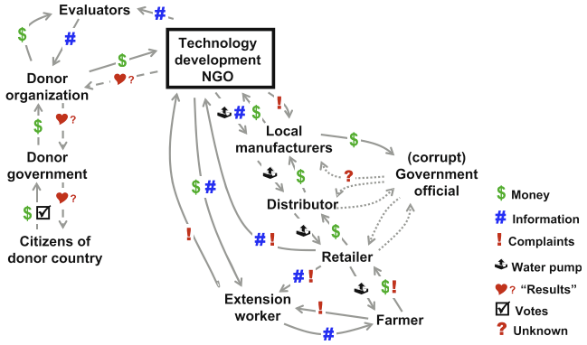
Case study 3: donor-funded micro-irrigation pump

This paper presents three interrelated frameworks as a first attempt to define the fundamentals of service systems.

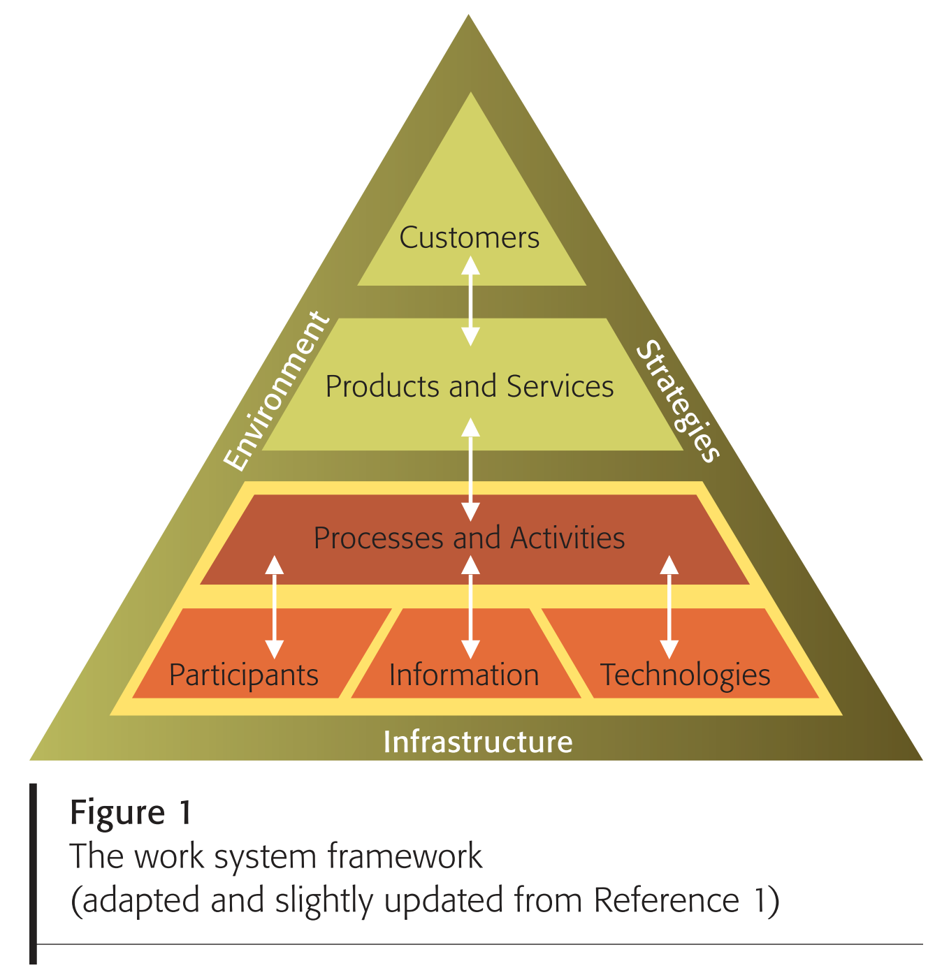
  • The work system framework uses nine basic elements to provide a system-oriented view of any system that performs work within or across organizations. Service systems are work systems.
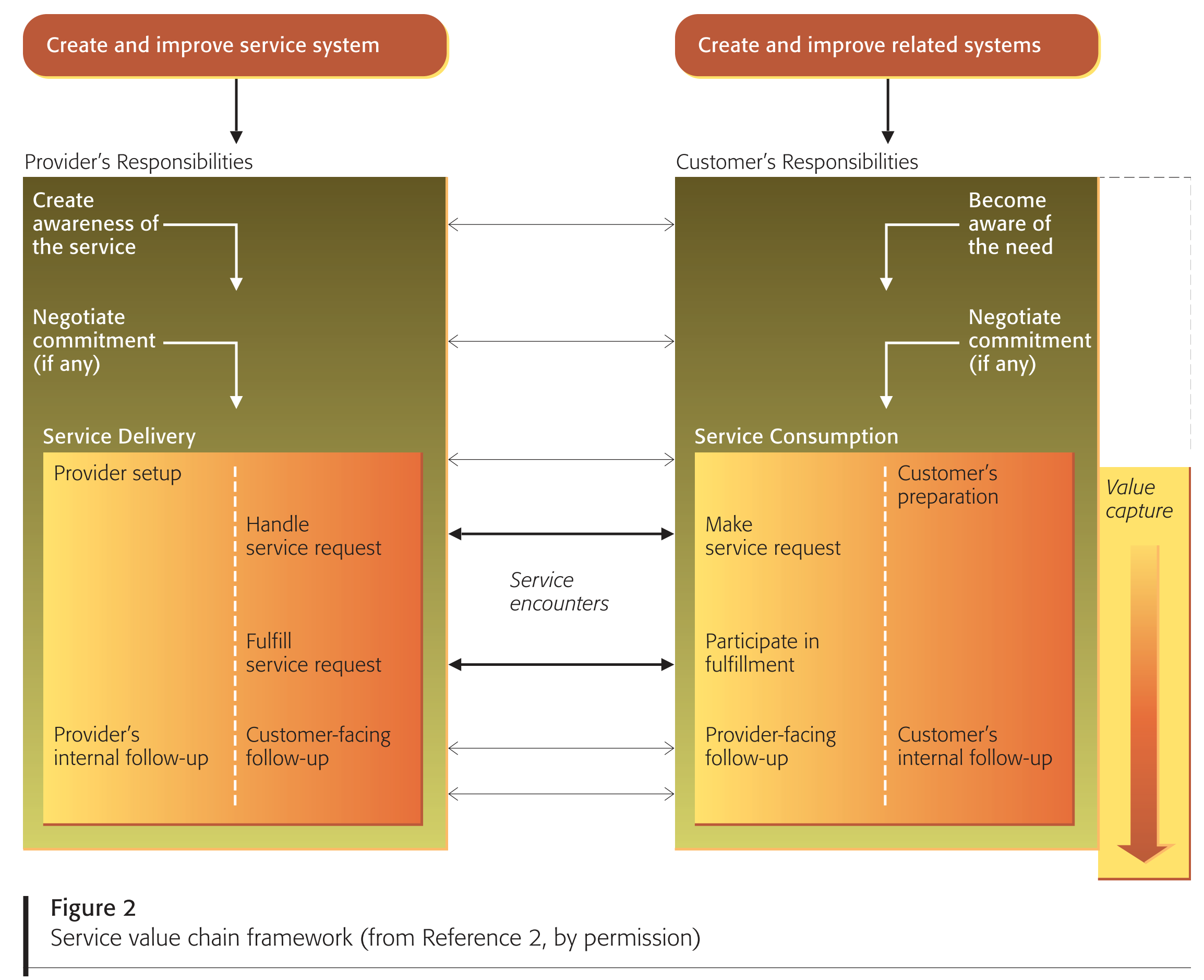
  • The service value chain framework augments the work system framework by introducing functions that are associated specifically with services. It presents a two-sided view of service processes based on the common observation that services are typically coproduced by service providers and customers.
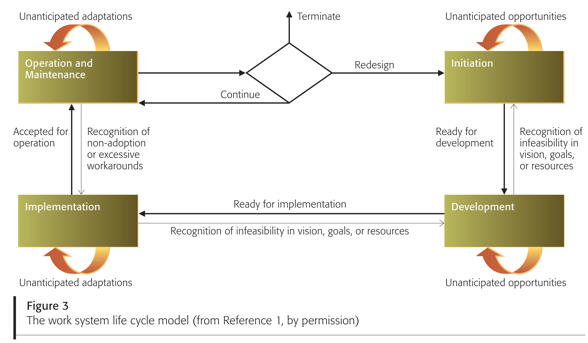
  • The work system life cycle model looks at how work systems (including service systems) change and evolve over time. It treats the life cycle of a system as a set of iterations involving planned and unplanned change.

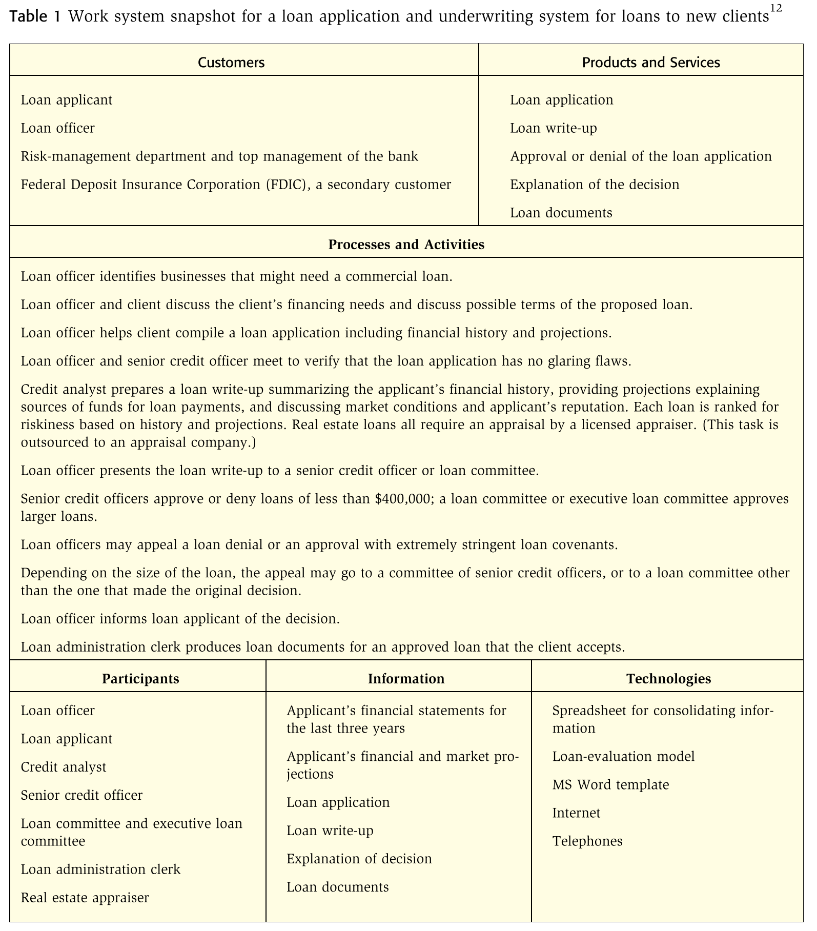
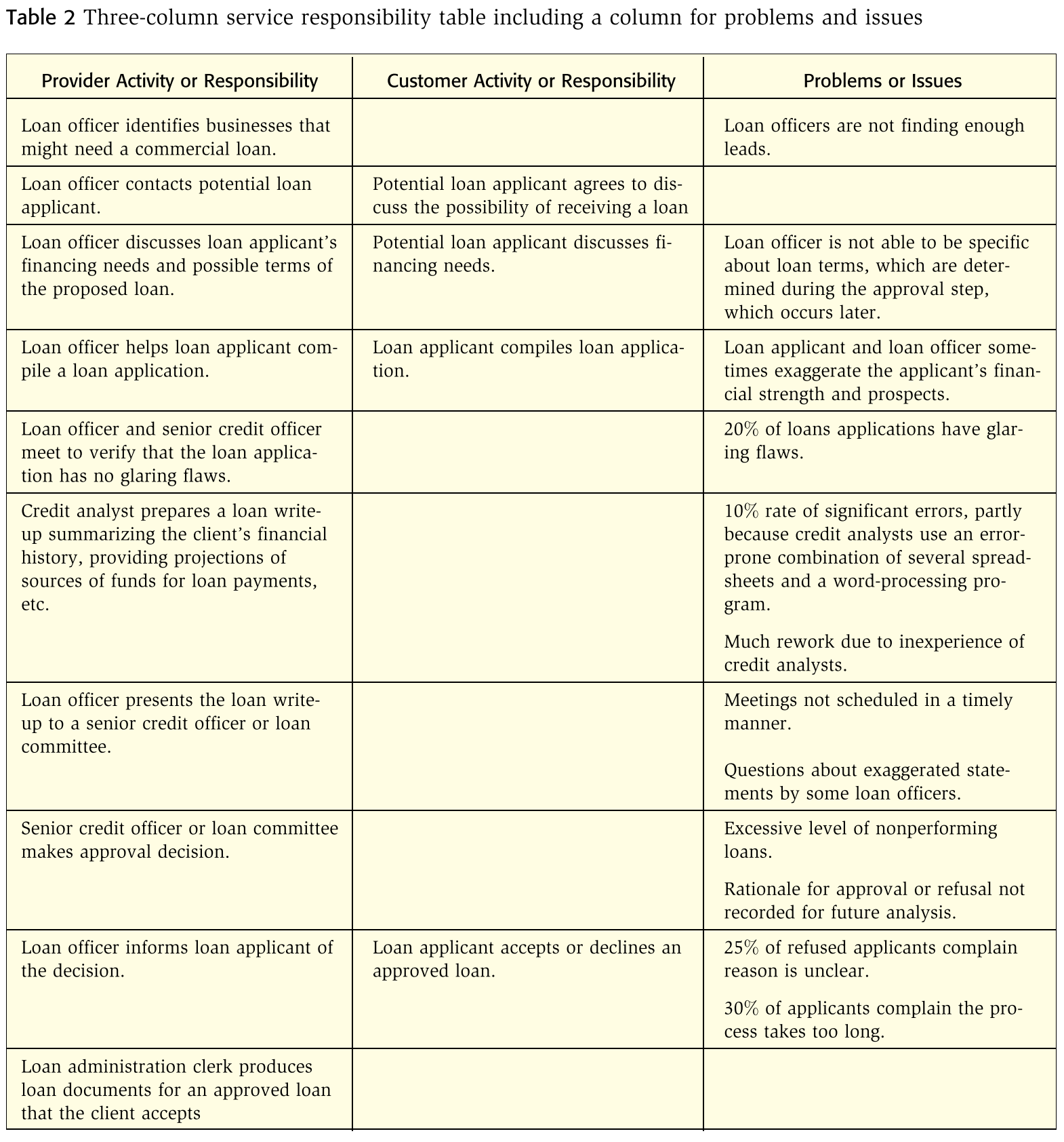
This paper uses two examples, one largely manual and one highly automated, to illustrate the potential usefulness of the three frameworks, which can be applied together to describe, analyze, and study how service systems are created, how they operate, and how they evolve through a combination of planned and unplanned change.

BPMN2.0入门到精通,这一篇就够了

笔者默认看这篇文章的同学都是了解、知道什么是BPMN的,因此背景知识、历史发展什么的都直接略过,我们直切正题:BPMN中的五个基础元素类别。

  1. 流对象(Flow Objects):流对象是定义业务流程的主要图形元素,主要有三种流对象
    1. 事件(Events)
    2. 活动(Activities)
    3. 网关(Gateways)
  2. 数据(Data):数据主要通过四种元素表示
    1. 数据对象(Data Objects)
    2. 数据输入(Data Inputs)
    3. 数据输出(Data Outputs)
    4. 数据存储(Data Stores)
  3. 连接对象(Connecting Objects):流对象彼此互相连接或者连接到其他信息的方法主要有四种
    1. 顺序流(Sequence Flows)
    2. 信息流(Message Flows)
    3. 协同(Associations)
    4. 数据协同(Data Associations)
  4. 泳道(Swimlanes):有两种方式通过泳道对主要的建模元素进行分组
    1. 泳池:Pools
    2. 泳道:Lanes
  5. Artifacts:主要用来提供关于流程的额外信息。BPMN2.0定义两种标准Artifacts,但是建模者或者建模工具可以增加任意多Artifacts。(Artifacts,有的地方翻译成“工件”,但是感觉不管翻译成什么都不够传神,所以本文中就不翻译这个词了。)
    1. 组:Group
    2. 文本注释:Text Annotation

流对象(Flow Objects)

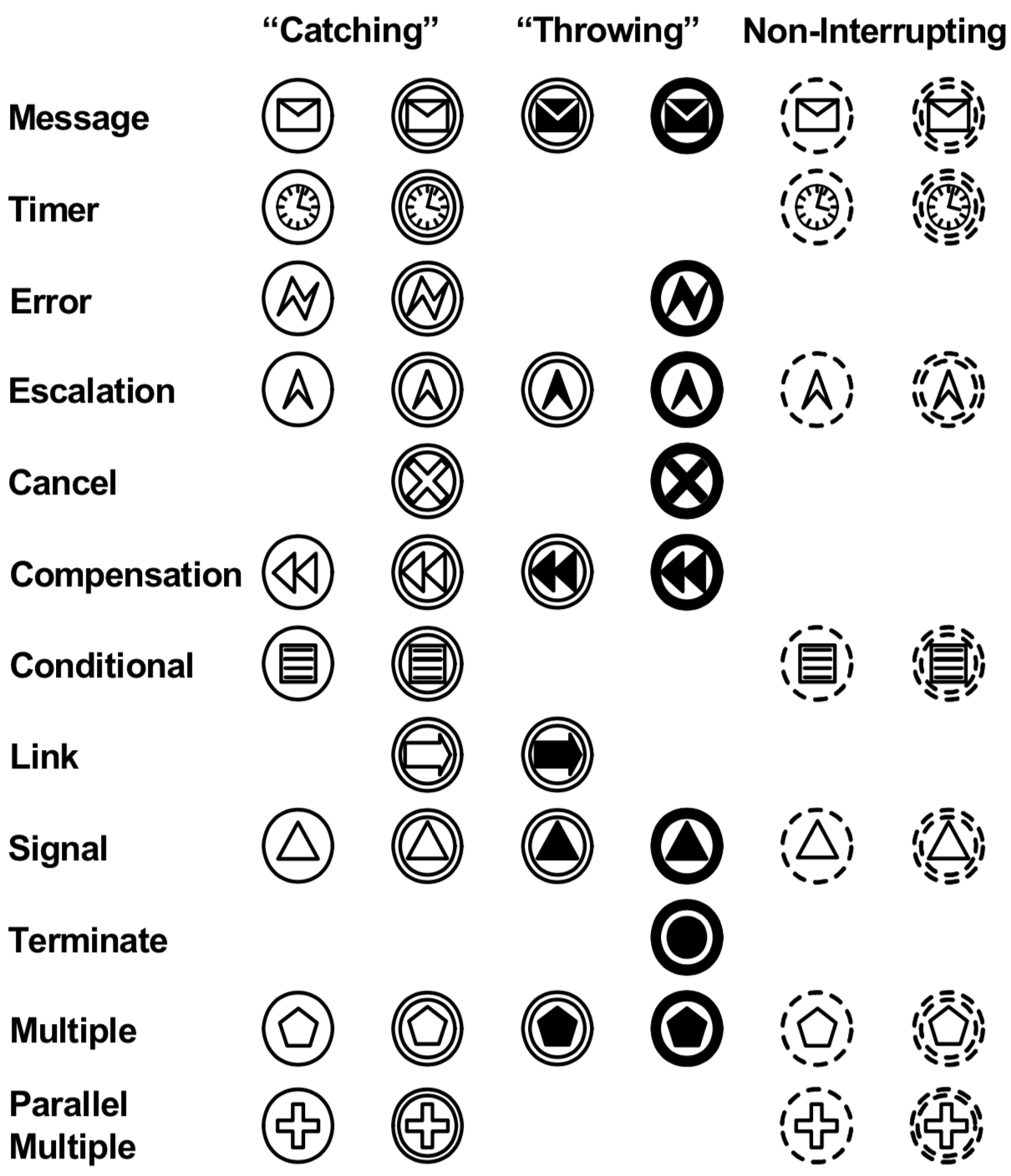
事件(Event)

元素 Element 描述 Description 符号 Notation
开始事件 Start 表示一个流程(Process)或一个编排(choreography)的开始
中间事件 Intermediate 发生在开始和结束事件之间,影响处理流程
结束事件 End 表示一个流程(Process)或一个编排(choreography)的结束
其他 开始事件和一些中间事件具有定义事件原因的“触发器”。结束事件可以定义作为序列流路径结束的“结果”。开始事件只能对触发器(“catch”)做出反应。结束事件只能创建(“抛出”)结果。中间事件可以捕获或抛出触发器。对于捕获的事件、触发器,标记未填充;对于抛出的触发器和结果,标记已填充。另外,在bpmn 1.1中用来中断活动的一些事件现在可以在不中断的模式下使用。这些事件的边界是虚线(见右图)。

活动(Activity)

元素 Element 描述 Description 符号 Notation
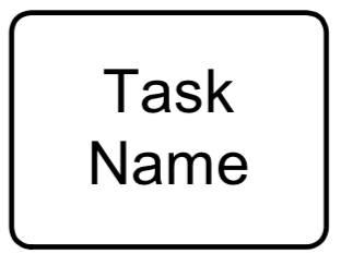
活动 Activity 活动是公司在流程中执行的工作的通用术语。活动可以是原子的或非原子的(聚合物)。作为流程模型一部分的活动类型有:子流程和任务,它们都是圆角矩形。活动用于标准流程Process和编排Choreography。
任务(原子) Task(atomic) 任务是包含在流程中的原子活动。任务是当流程中的工作无法分解为更精细的流程细节级别时使用。
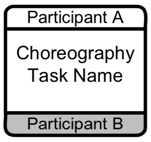
编排任务 Choreography Task 表示一个或多个消息交换的集合。每个编排任务涉及两个参与者。
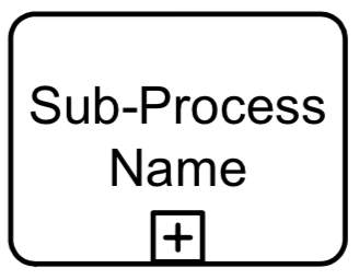
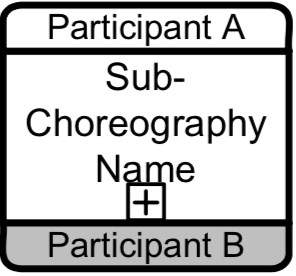
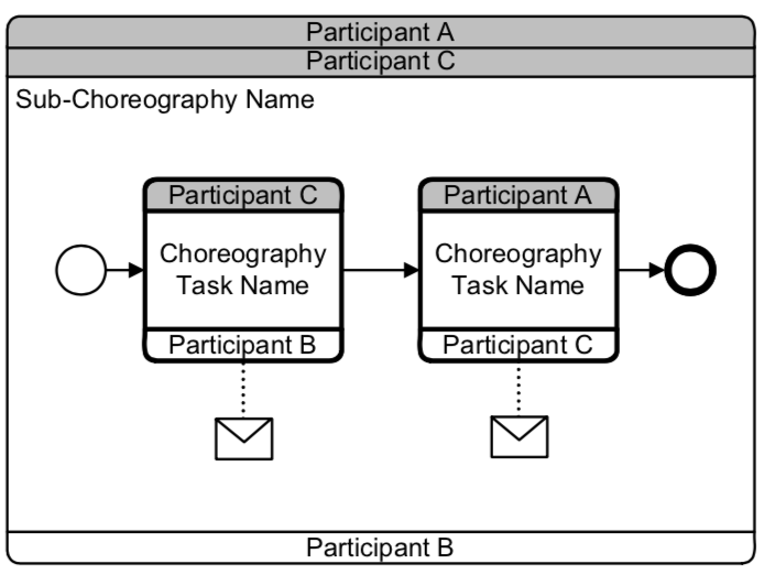
子流程 Sub-Process 子流程是包含在流程或编排中的复合活动。它是复合的,因为它可以通过一组子活动分解为更细粒度级别的流程或编排。子流程活动主要有以下四类 Collapsed Sub-ProcessExpanded Sub-ProcessCollapsed Sub- ChoreographyExpanded Sub-Choreography

网关(Gateway)

元素 Element 描述 Description 符号 Notation
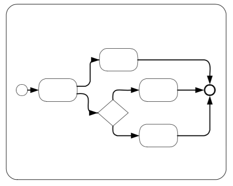
网关 Gateway 网关用于顺序流程和编排中序列流的发散和收敛。因此,它将决定路径的分支、分叉、合并和连接。内部标记将指示行为控制的类型(见下边一行)。
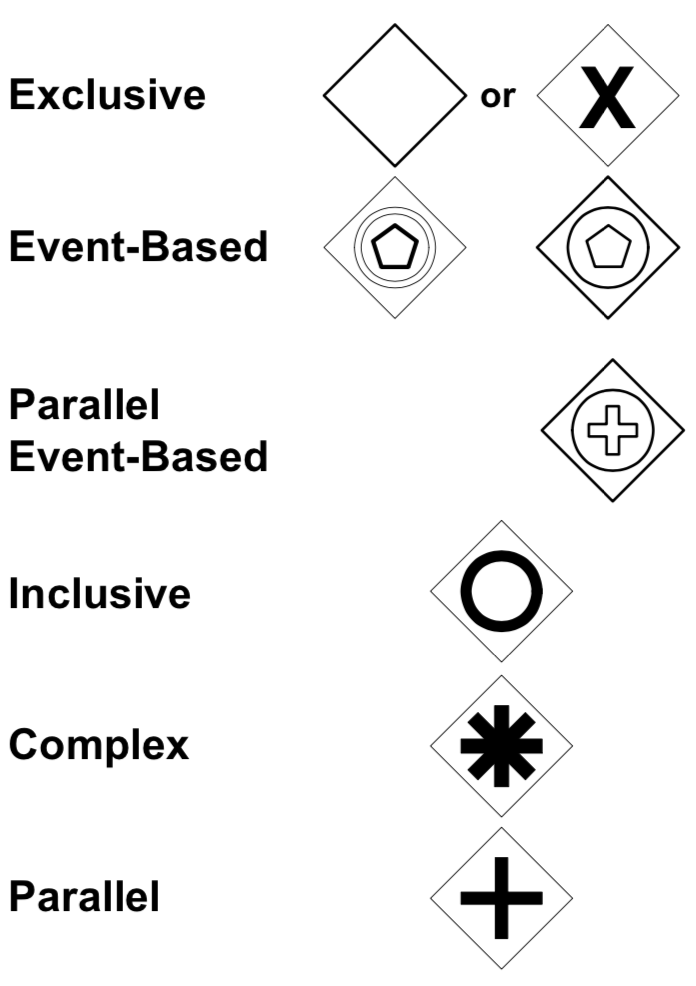
网关控制类型 Gateway Control Type 网关菱形内的图标将指示流控制行为的类型。控制类型包括:•排他型exclusive决策和合并。排他型exclusive和基于事件event-based的网关都执行排他决策,合并排他可以使用或不使用“x”标记来显示。•基于事件event-based和基于并行事件parallel event-based的网关可以启动流程的新实例。•包容型inclusive网关决策和合并。•复杂型complex网关——复杂的条件和情况。•并行parallel网关分叉和连接。每种类型的控件都会影响传入和传出流。

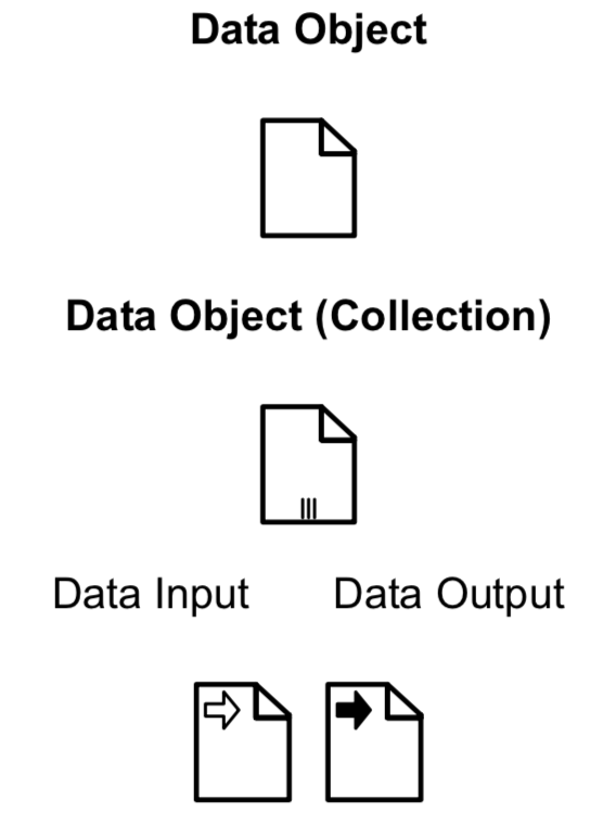
数据(Data)

数据对象提供有关需要执行的活动和/或它们产生的内容的信息,数据对象可以表示单个数据对象或数据对象集合。数据输入和数据输出为流程提供相同的信息。

连接对象(Connecting Objects)

元素 Element 描述 Description 符号 Notation
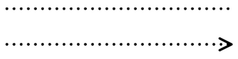
顺序流 Sequence Flow 表示活动的执行顺序
信息流 Message Flow 表示两个参与者之间准备发送和接收的信息流
协同 Association 协同用于将信息和artifact与图形元素链接。如果有箭头,则表示流向(如数据)。

泳道(Swimlanes)

元素 Element 描述 Description 符号 Notation
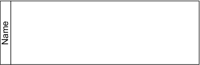
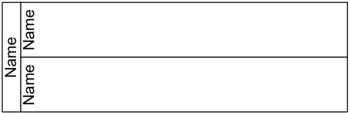
泳池 Pool 泳池是协作中参与者的图形表示。它还充当一个“泳道”和一个图形容器,用于从其他池中分割一组活动,通常是在B2B环境中。泳池可以具有内部详细信息,以将要执行的进程的形式显示。或者一个泳池可能没有内部细节,也就是说,它可以是一个“黑匣子”。
泳道 Lane lane是进程中的一个子分区,有时在泳池中,它将垂直或水平地扩展进程的整个长度。泳道用于组织和分类活动。

Artifacts

元素 Element 描述 Description 符号 Notation
组 Group 组是同一类别内的图形元素的组。这种类型的分组不影响组内的序列流。类别名称在关系图上显示为组标签。类别可用于文档或分析目的。组是可以在图表上直观显示对象类别的一种方式。
文本注释 Text Annotation 是一个帮助建模者给图形元素增加额外文本说明的机制。

总结

至此,你已经通过 20% 的时间了解了BPMN2.0 接近 80% 的内容。虽然BPMN底层语法以及结构还没有学习,但是这并不影响你已经可以通过BPMN2.0对你所在的业务进行详尽的描述!

Definition(定义)

A precise and unambiguous description of the meaning of a mathematical term. It characterizes the meaning of a word by giving all the properties and only those properties that must be true.

对数学术语含义的精确而明确的描述。它通过给出一个词的所有性质,仅给出那些必须为真的性质,来表征该词的意义。

Theorem(定理)

A mathematical statement that is proved using rigorous mathematical reasoning. In a mathematical paper, the term theorem is often reserved for the most important results.

用严格的数学推理证明的数学陈述。在数学论文中,术语定理通常是为最重要的结果而保留的。

Lemma(引理)

A minor result whose sole purpose is to help in proving a theorem. It is a stepping stone on the path to proving a theorem. Very occasionally lemmas can take on a life of their own.

唯一目的是帮助证明定理的小结果。这是证明一个定理之路的踏脚石。极少情况下引理可以独立存在。

Corollary(推论)

A result in which the (usually short) proof relies heavily on a given theorem (we often say that “this is a corollary of Theorem A”).

证明(通常是简短的)很大程度上依赖于一个给定定理的结果(我们经常说“这是定理A的一个推论”)。

Proposition(命题)

A proved and often interesting result, but generally less important than a theorem.

一个被证明的,通常很有趣的结果,但一般没有定理重要。

Conjecture(推测,猜想)

A statement that is unproved, but is believed to be true.

Claim(断言)

An assertion that is then proved. It is often used like an informal lemma.

未经证实但被认为是真实的陈述。

Axiom/Postulate(公理/假定)

A statement that is assumed to be true without proof. These are the basic building blocks from which all theorems are proved.

没有证明,且假设为真的陈述。这些是证明所有定理的基本构造块。

Identity(恒等式)

A mathematical expression giving the equality of two (often variable) quantities.

两个(通常是可变的)量相等的数学表达式。

Paradox(悖论)

A statement that can be shown, using a given set of axioms and de nitions, to be both true and false. Paradoxes are often used to show the  inconsistencies in an awed theory. The term paradox is often used informally to describe a surprising or counterintuitive result that follows from a given set of rules.

一种使用一组给定的公理和定义,既正确又错误的陈述。悖论经常被用来显示敬畏理论中的矛盾。“悖论”一词通常被非正式地用来描述从一组给定规则得出的令人惊讶或违反直觉的结果。